deepsense.io announced the launch of Neptune – its innovative machine learning platform for managing multiple data science experiments. The premiere took place at the inaugural A.I. Conference (September 26-27) as well as this year’s Strata + Hadoop World (September 27-29), both being held in New York City.
Neptune simplifies the process of managing and monitoring machine learning experiments, freeing data science teams to focus on the substance of their work rather than complex and time-consuming organizational tasks. Neptune was originally developed as an in-house tool to assist deepsense.io’s award-winning machine learning team in its work on complex data science projects. Neptune’s powerful Web UI and useful for scripting CLIs allow teams to monitor long-running experiments and simplify group collaboration. With deepsense.io’s new machine learning platform, data science research and software engineering teams have instant access and control over each experiment. Neptune automatically stores the entire environment needed to rerun each experiment and its related artifacts for browsing and comparing, and each experiment’s execution can be monitored with real-time metrics and may be aborted at any time.
“In order to create a state-of-the-art machine learning model, data scientists have to conduct hundreds of experiments. Each experiment is related to different source code, depends on different input data and is run on different infrastructure. All of this makes data scientists’ everyday work very hard to organize and, as a result, highly inefficient,” explains Piotr Niedzwiedz, CTO at deepsense.io. “That’s why we originally developed Neptune for our machine learning team. When we saw that it worked perfectly for us, we decided to provide its capabilities to other data science teams struggling with similar problems. And now, we are ready to introduce Neptune on the global market.”
https://deepsense.ai/wp-content/uploads/2019/02/world-premiere-of-neptune-deepsense-ios-new-machine-learning-platform-for-managing-data-science-experiments.jpg3371140Barbara Rutkowskahttps://deepsense.ai/wp-content/uploads/2023/10/Logo_black_blue_CLEAN_rgb.pngBarbara Rutkowska2016-09-28 12:21:572019-07-26 09:14:06World premiere of Neptune – deepsense.io’s new machine learning platform for managing data science experiments
Latest version of deepsense.io’s flagship Big Data product now features Spark 2.0 support, external Spark clusters, and custom operations and notebooks in R.
deepsense.io is proud to announce the launch of Seahorse 1.3, the latest version of its scalable data analytics workbench powered by Apache Spark, at Strata+Hadoop World NY 2016 conference. Seahorse allows data scientists to visually design, edit and execute Spark applications using a Web-based, code-free UI.
New features in Seahorse 1.3 include: support for Spark 2.0, quick and easy connections to external Spark clusters, custom operations and Notebooks in R and a file library. These improvements will allow data scientists to benefit from up to 10x query speed-up, the ability to quickly connect to and work on multiple external clusters, improved expressiveness with R code snippets and Notebooks as well as, easier transfer of files between local machines and Spark clusters.
Download your copy of Seahorse 1.3 here.
Seahorse 1.3 is available as an app on Trusted Analytics Platform (TAP) and IBM’s Data Scientist Workbench, two of the world’s most popular open-source platforms for advanced analytics and machine learning solutions.
deepsense.io will unveil Seahorse, release 1.3 at the Strata+Hadoop World Conference 2016 to be held at New York City’s Javits Center. During the conference, deepsense.io will also announce its brand-new product – Neptune – an IT platform-based machine learning experiment management solution for data scientists.
Spark Summit 2016 San Francisco will take place from June 6-8, 2016 at the Hilton San Francisco Union Square, 333 O’Farrell St., San Francisco, CA 94102.
###
About deepsense.ai:
Media contact:
deepsense.ai trademarks at boilerplate
https://deepsense.ai/wp-content/uploads/2019/02/deepsense-io-announces-seahorse-1-3-release-at-2016-stratahadoop-world-ny.jpg3371140Barbara Rutkowskahttps://deepsense.ai/wp-content/uploads/2023/10/Logo_black_blue_CLEAN_rgb.pngBarbara Rutkowska2016-09-27 12:21:232019-07-26 09:13:58deepsense.io announces Seahorse 1.3 release at 2016 Strata+Hadoop World NY
In 2013 the Deepmind team invented an algorithm called deep Q-learning. It learns to play Atari 2600 games using only the input from the screen. Following a call by OpenAI, we adapted this method to deal with a situation where the playing agent is given not the screen, but rather the RAM state of the Atari machine. Our work was accepted to the Computer Games Workshop accompanying the IJCAI 2016 conference. This post describes the original DQN method and the changes we made to it. You can re-create our experiments using a publicly available code.
Atari games
Atari 2600 is a game console released in the late 1970s. If you were a lucky teenager at that time, you would connect the console to the TV-set, insert a cartridge containing a ROM with a game and play using the joystick. Even though the graphics were not particularly magnificent, the Atari platform was popular and there are currently around \(400\) games available for it. This collection includes immortal hits such as Boxing, Breakout, Seaquest and Space Invaders.
agent (which sees states and rewards and decides on actions) and
environment (which sees actions, changes states and gives rewards).
R. Sutton and A. Barto: Reinforcement Learning: An Introduction
In our case, the environment is the Atari machine, the agent is the player and the states are either the game screens or the machine’s RAM states. The agent’s goal is to maximize the discounted sum of rewards during the game. In our context, “discounted” means that rewards received earlier carry more weight: the first reward has a weight of \(1\), the second some \(gamma\) (close to \(1\)), the third \(gamma^2\) and so on.
Q-values
Q-value (also called action-value) measures how attractive a given action is in a given state. Let’s assume that the agent’s strategy (the choice of the action in a given state) is fixed. Then a Q-value of a state-action pair \((s, a)\) is the cumulative discounted reward the agent will get if it is in a state \(s\), executes the action \(a\) and follows his strategy from there on.
The Q-value function has an interesting property – if a strategy is optimal, the following holds:
$$
Q(s_t, a_t) = r_t + gamma max_a Q(s_{t+1}, a)
$$
One can mathematically prove that the reverse is also true. Namely, any strategy which satisfies the property for all state-action pairs is optimal. This fact is not restricted to deterministic strategies. For stochastic strategies, you have to add some expectation value signs and all the results still hold.
Q-learning
The above concept of Q-value leads to an algorithm learning a strategy in a game. Let’s slowly update the estimates of the state-action pairs to the ones that locally satisfy the property and change the strategy, so that in each state it will choose an action with the highest sum of expected reward (estimated as an average reward received in a given state after following given action) and biggest Q-value of the subsequent state.
for all (s,a):
    Q[s, a] = 0 #initialize q-values of all state-action pairs
for all s:
    P[s] = random_action() #initialize strategy
# assume we know expected rewards for state-action pairs R[s, a] and
# after making action a in state s the environment moves to the state next_state(s, a)
# alpha : the learning rate - determines how quickly the algorithm learns;
#                             low values mean more conservative learning behaviors,
#                             typically close to 0, in our experiments 0.0002
# gamma : the discount factor - determines how we value immediate reward;
#                               higher gamma means more attention given to far-away goals
#                               between 0 and 1, typically close to 1, in our experiments 0.95
repeat until convergence:
  1. for all s:
         P[s] = argmax_a (R[s, a] + gamma * max_b(Q[next_state(s, a), b]))
  2. for all (s, a):
         Q[s, a] = alpha*(R[s, a] + gamma * max_b Q[next_state(s, a), b]) + (1 - alpha)Q[s, a]
This algorithm is called Q-learning. It converges in the limit to an optimal strategy. For simple games like Tic-Tac-Toe, this algorithm, without any further modifications, solves them completely not only in theory but also in practice.
Deep Q-learning
Q-learning is a correct algorithm, but not an efficient one. The number of states which need to be visited multiple times to learn their action-values is too big. We need some form of generalization: when we learn about the value of one state-action pair, we can also improve our knowledge about other similar state-actions.
The deep Q-learning algorithm uses the convolutional neural network as a function approximating the Q-value function. It accepts the screen (after some transformations) as an input. The algorithm transforms the input with a couple of layers of nonlinear functions. Then it returns an up to \(18\) dimensional vector. Entries of the vector denote the approximated Q-values of the current state and each of the possible actions. The action to choose is the one with the highest Q-value.
Training consists of playing the episodes of the game, observing transitions from state to state (doing the currently best actions) and rewards. Having all this information, we can estimate the error, which is the square of the difference between the left- and right-hand side of the Q-learning property above:
$$
error = (Q(s_t, a_t) – (r_t + gamma max_a Q(s_{t+1}, a)))^2
$$
We can calculate the gradient of this error according to the network parameters and update them to decrease the error using one of the many gradient descent optimization algorithms (we used RMSProp).
DQN+RAM
In our work, we adapted the deep Q-learning algorithm so that its input are not game screens, but the RAM states of the Atari machine. Atari 2600 has only \(128\) bytes of RAM. On one hand, this makes our task easier, as our input is much smaller than the full screen of the console. On the other hand, the information about the game may be hard to retrieve. We tried two network architectures. One with \(2\) hidden ReLU layers, \(128\) nodes each, and the other with \(4\) such layers. We obtained results comparable (in two games higher, in one lower) to those achieved with the screen input in the original DQN paper. Admittedly, higher scores can be achieved using more computational resources and some additional tricks.
Tricks
The method of learning Atari games, as presented above and even with neural networks employed to approximate the Q-values, would not yield good results. To make it work, the original DQN paper’s authors and we in our experiments, employed a few improvements to the basic algorithm. In this section, we discuss some of them.
Epsilon-greedy strategy
When we begin our agent’s training, it has little information about the value of particular game states. If we were to completely follow the learned strategy at the start of the training we’d be nearly randomly choosing some actions to follow in the first game states. As the training continues, we’d stick to these actions for the first states, as their value estimation would be positive (and for the other actions would be nearly zero). The value of the first-chosen action would improve and we’d only pick these, without even testing the other possibilities. The first decisions, made with little information, would be reinforced and followed in the future.
We say that such a policy doesn’t have a good exploration-exploitation tradeoff. On one hand, we’d like to focus on the actions that led to reasonable results in the past, but on the other ahnd, we prefer our policies to extensively explore the state-action space.
The solution to this problem used in DQN is using an epsilon-greedy strategy during training. This means that at any time with some small probability \(varepsilon\) the agent chooses a random action, instead of always choosing the action with the best Q-value in the given state. Then, every action will get some attention and its state-action value estimation will be based on some (possibly limited) experience and not the initialization values.
We join this method with epsilon decay — at the beginning of training we set \(varepsilon\) to a high value (\(1.0\)), meaning that we prefer to explore the various actions and gradually decrease \(varepsilon\) to a small value, that indicate the preference to exploit the well-learned action-values.
Experience replay
Another trick used in DQN is called experience replay. The process of training a neural network consist of training epochs; in each epoch we pass all the training data, in batches, as the network input and update the parameters based on the calculated gradients.
When training reinforcement learning models, we don’t have an explicit dataset. Instead, we experience some states, actions, and rewards. We pass them to the network, so that our statistical model can learn what to do in similar game states. As we want to pass a particular state/action/reward tuple multiple times to the network, we save them in memory when they are seen. To fit this data to the RAM of our GPU, we store at most \(100 000\) recently observed state/action/reward/next state tuples.
When the dataset is queried for a batch of training data, we don’t return consecutive states, but a set of random tuples. This reduces correlation between states processed in a given step of learning. As a result, this improves the statistical properties of the learning process.
For more details about experience replay you can see Section 3.5 of Lin’s thesis. As quite a few other tricks in reinforcement learning, this method was invented back in 1993 – significantly before the current deep learning boom.
Frameskip
Atari 2600 was designed to use an analog TV as the output device. The console generated \(60\) new frames appearing on the screen every second. To simplify the search space we imposed a rule that one action is repeated over a fixed number of frames. This fixed number is called the frame skip. The standard frame skip used in the original work on DQN is \(4\). For this frame skip the agent makes a decision about the next move every \( 4cdot frac{1}{60} = frac{1}{15}\) of a second. Once a decision is made, it remains unchanged during the next \(4\) frames. A low frame skip allows the network to learn strategies based on a super-human reflex. A high frame skip will limit the complexity of a strategy. Hence learning may be faster and more successful whenever strategy matters over tactic. In our work , we tested frame skips equal to \(4,8\) and \(30\).
https://deepsense.ai/wp-content/uploads/2019/02/Playing-Atari-games-using-RAM-state.jpg3371140Henryk Michalewskihttps://deepsense.ai/wp-content/uploads/2023/10/Logo_black_blue_CLEAN_rgb.pngHenryk Michalewski2016-09-27 12:00:342023-02-28 21:57:21Playing Atari on RAM with Deep Q-learning
In January 2016, deepsense.ai won the Right Whale Recognition contest on Kaggle. The competition’s goal was to automate the right whale recognition process using a dataset of aerial photographs of individual whales. The terms and conditions for the competition stated that to collect the prize, the winning team had to provide source code and a description of how to recreate the winning solution. A fair request, but as it turned out, the winning solution’s authors spent about three weeks recreating all of the steps that led them to the winning machine learning model.
When data scientists work on a problem, they need to test many different approaches – various algorithms, neural network structures, numerous hyperparameter values that can be optimized etc. The process of validating one approach can be called an experiment. The inputs for every experiment include: source code, data sets, hyperparameter values and configuration files. The outputs of every experiment are: output model weights (definition of the model), metric values (used for comparing different experiments), generated data and execution logs. As we can see, that’s a lot of different artifacts for each experiment. It is crucial to save all of these artifacts to keep track of the project – comparing different models, determining which approaches were already tested, expanding research from some experiment from the past etc. Managing the process of experiment executions is a very hard task and it is easy to make a mistake and lose an important artifact.
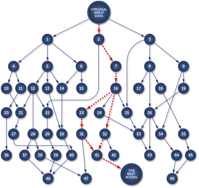
To make the situation even more complicated, experiments can depend on each other. For example, we can have two different experiments training two different models and a third experiment that takes these two models and creates a hybrid to generate predictions. Recreating the best solution means finding the path from the original data set to the model that gives the best results.
Recreating the path that led to the best model
The deepsense.ai research team performed around 1000 experiments to find the competition-winning solution. Knowing all that, it becomes clear why recreating the solution was such a difficult and time consuming task.
The problem of recreating a machine learning solution is present not only in an academic environment. Businesses struggle with the same problem. The common scenario is that the research team works to find the best machine learning model to solve a business problem, but then the software engineering team has to put the model into a production environment. The software engineering team needs a detailed description of how to recreate the model.
Our research team needed a platform that would help them with these common problems. They defined the properties of such a platform as:
Every experiment and the related artifacts are registered in the system and accessible for browsing and comparing;
Experiment execution can be monitored via real-time metrics;
Experiment execution can be aborted at any time;
Data scientists should not be concerned with the infrastructure for the experiment execution.
deepsense.ai decided to build Neptune – a brand new machine learning platform that organizes data science processes. This platform relieves data scientists of the manual tasks related to managing their experiments. It helps with monitoring long-running experiments and supports team collaboration. All these features are accessible through the powerful Neptune Web UI and useful for scripting CLI.
Neptune is already used in all machine learning projects at deepsense.ai. Every week, our data scientists execute around 1000 experiments using this machine learning platform. Thanks to that, the machine learning team can focus on data science and stop worrying about process management.
Experiment Execution in Neptune
Main Concepts of the Machine Learning Platform
Job
A job is an experiment registered in Neptune. It can be registered for immediate execution or added to a queue. The job is the main concept in Neptune and contains a complete set of artifacts related with the experiment:
source code snapshot: Neptune creates a snapshot of the source code for every job. This allows a user to revert to any job from the past and get the exact version of the code that was executed;
parameters: customly defined by a user. Neptune supports boolean, numeric and string types of parameters;
data and logs generated by the job;
metric values represented as channels.
Neptune is library and framework agnostic. Users can leverage their favorite libraries and frameworks with Neptune. At deepsense.ai we currently execute Neptune jobs that use: TensorFlow, Theano, Caffe, Keras, Lasagne or scikit-learn.
Channel
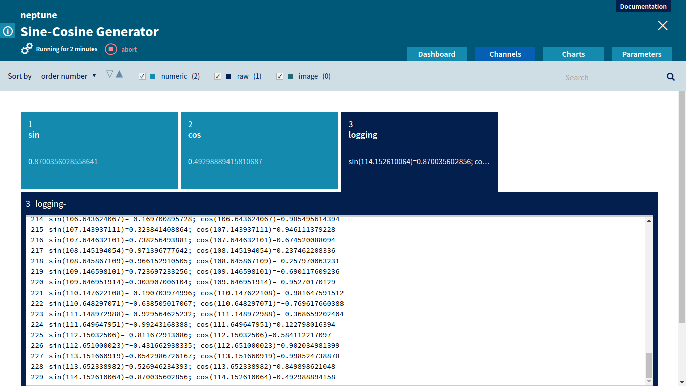
A channel is a mechanism for real-time job monitoring. In the source code, a user can create channels, send values through them and then monitor these values live using the Neptune Web UI. During job execution, a user can see how his or her experiment is performing. The Neptune machine learning platform supports three types of channels:
Numeric: used for monitoring any custom-defined metric. Numeric channels can be displayed as charts. Neptune supports dynamic chart creation from the Neptune Web UI with multiple channels displayed in one chart. This is particularly useful for comparing various metrics;
Text: used for logs;
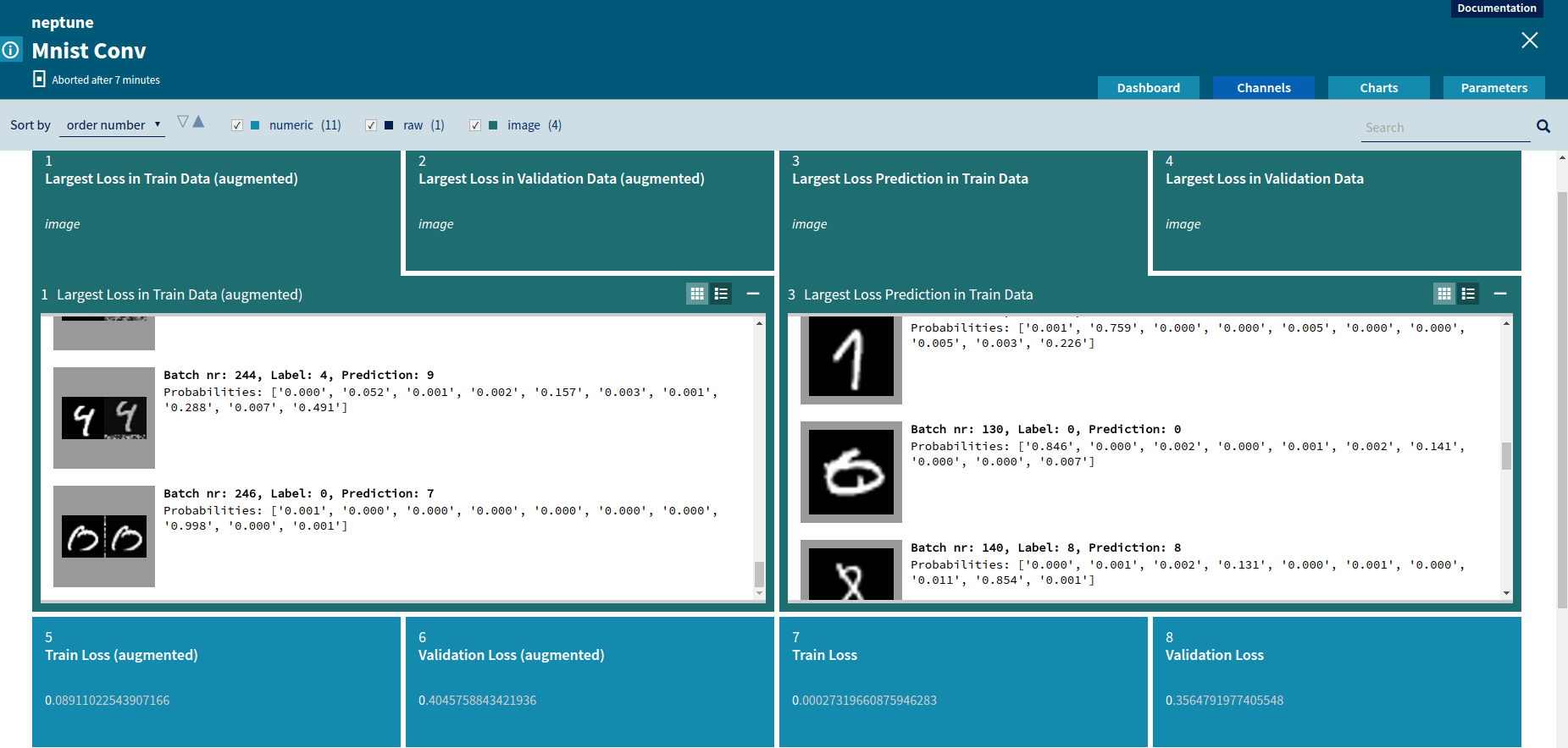
Image: used for sending images. A common use case for this type of channel is checking the behavior of an applied augmentation when working with images.
Comparing two Neptune image channels
Queue
A queue is a very simple mechanism that allows a user to execute his or her job on remote infrastructure. A common setup for many research teams is that data scientists develop their code on local machines (laptops), but due to hardware requirements (powerful GPU, large amount of RAM, etc) code has to be executed on a remote server or in a cloud. For every experiment, data scientists have to move source code between the two machines and then log into the remote server to execute the code and monitor logs. Thanks to our machine learning platform, a user can enqueue a job from a local machine (the job is created in Neptune, all metadata and parameters are saved, source code copied to users’ shared storage). Then, on a remote host that meets the job requirements the user can execute the job with a single command. Neptune takes care of copying the source code, setting parameters etc.
The queue mechanism can be used to write a simple script that queries Neptune for enqueued jobs and execute the first job from the queue. If we run this script on a remote server in an infinite loop, we don’t have to log to the server ever again because the script executes all the jobs from the queue and reports the results to the machine learning platform.
Creating a Job
Neptune is language and framework agnostic. A user can communicate with Neptune using REST API and Web Sockets from his or her source code written in any language. To make the communication easier, we provide a high-level client library for Python (other languages are going to be supported soon).
Let’s examine a simple job that provided with amplitude and sampling_rate generates sine and cosine as functions of time (in seconds).
import math
import time
from deepsense import neptune
ctx = neptune.Context()
amplitude = ctx.params.amplitude
sampling_rate = ctx.params.sampling_rate
sin_channel = ctx.job.create_channel(name='sin', channel_type=neptune.ChannelType.NUMERIC)
cos_channel = ctx.job.create_channel(name='cos', channel_type=neptune.ChannelType.NUMERIC)
logging_channel = ctx.job.create_channel(name='logging', channel_type=neptune.ChannelType.TEXT)
ctx.job.create_chart(name='sin & cos chart', series={'sin': sin_channel, 'cos': cos_channel})
ctx.job.finalize_preparation()
# The time interval between samples.
period = 1.0 / sampling_rate
# The initial timestamp, corresponding to x = 0 in the coordinate axis.
zero_x = time.time()
iteration = 0
while True:
    iteration += 1
    # Computes the values of sine and cosine.
    now = time.time()
    x = now - zero_x
    sin_y = amplitude * math.sin(x)
    cos_y = amplitude * math.cos(x)
    # Sends the computed values to the defined numeric channels.
    sin_channel.send(x=x, y=sin_y)
    cos_channel.send(x=x, y=cos_y)
    # Formats a logging entry.
    logging_entry = "sin({x})={sin_y}; cos({x})={cos_y}".format(x=x, sin_y=sin_y, cos_y=cos_y)
    # Sends a logging entry.
    logging_channel.send(x=iteration, y=logging_entry)
    time.sleep(period)
The first thing that we can see is that we need to import Neptune library and create a neptune.Context object. The Context object is an entrypoint for Neptune integration. Afterwards, using the context we obtain values for job parameters: amplitude and sampling_rate.
Then, using neptune.Context.job we create numeric channels for sending sine and cosine values and a text channel for sending logs. We want to display sin_channel and cos_channel on a chart, so we use neptune.Context.job.create_chart to define a chart with two series named sin and cos. After that, we need to tell Neptune that the preparation phase is over and we are starting the proper computation. That is what: ctx.job.finalize_preparation() does.
In an infinite loop we calculate sine and cosine functions values and send these values to Neptune using the channel.send method. We also create a human-readable log and send it through logging_channel.
To run main.py as a Neptune job we need to create a configurtion file – a descriptor file with basic metadata for the job.
config.yaml contains basic information about the job: name, project, owner and parameter definitions. For our simple Sine-Cosine Generator we need two parameters of double type: amplitude and sampling_rate (we already saw in the main.py how to obtain parameter values in the code).
To run the job we need to use the Neptune CLI command: neptune run main.py –config config.yaml –dump-dir-url my_dump_dir — –amplitude 5 –sampling_rate 2.5
For neptune run we specify: the script that we want to execute, the configuration for the job and a path to a directory where snapshot of the code will be copied to. We also pass values of the custom-defined parameters.
Job Monitoring
Every job executed in the machine learning platform can be monitored in the Neptune Web UI. A user can see all useful information related to the job:
metadata (name, description, project, owner);
job status (queued, running, failed, aborted, succeeded);
location of the job source code snapshot;
location of the job execution logs;
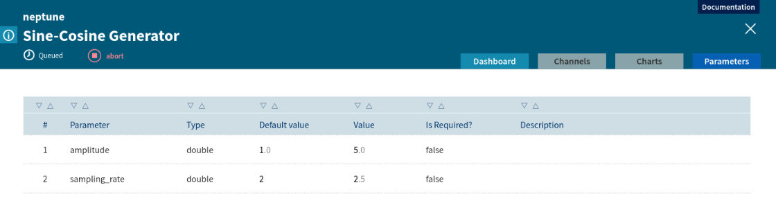
parameter schema and values.
Parameters for Sine-Cosine Generator
A data scientist can monitor custom metrics sent to Neptune through the channel mechanism. Values of the incoming channels are displayed in the Neptune Web UI in real time. If the metrics are not satisfactory, the user can decide to abort the job. Aborting the job can also be done from the Neptune Web UI.
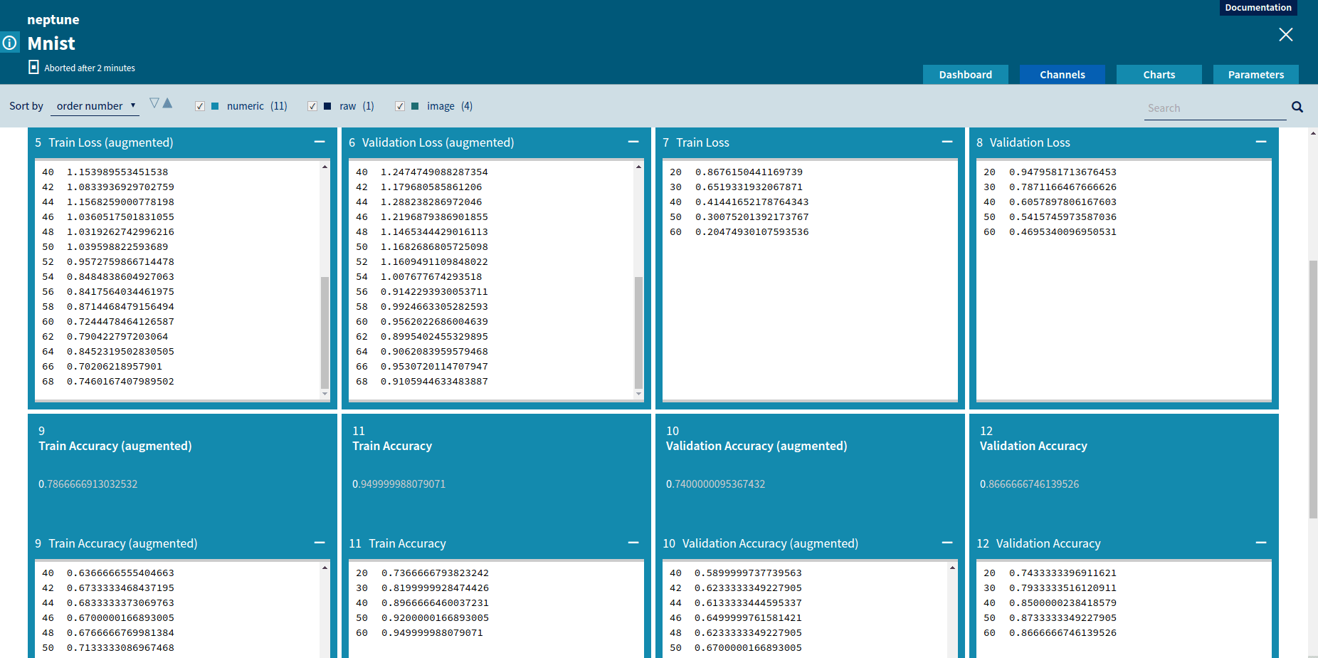
Channels for Sine-Cosine GeneratorComparing values of multiple metrics using Neptune channels
Numeric channels can be displayed graphically as charts. A chart representation is very useful to compare various metrics and to track changes of metrics during job execution.
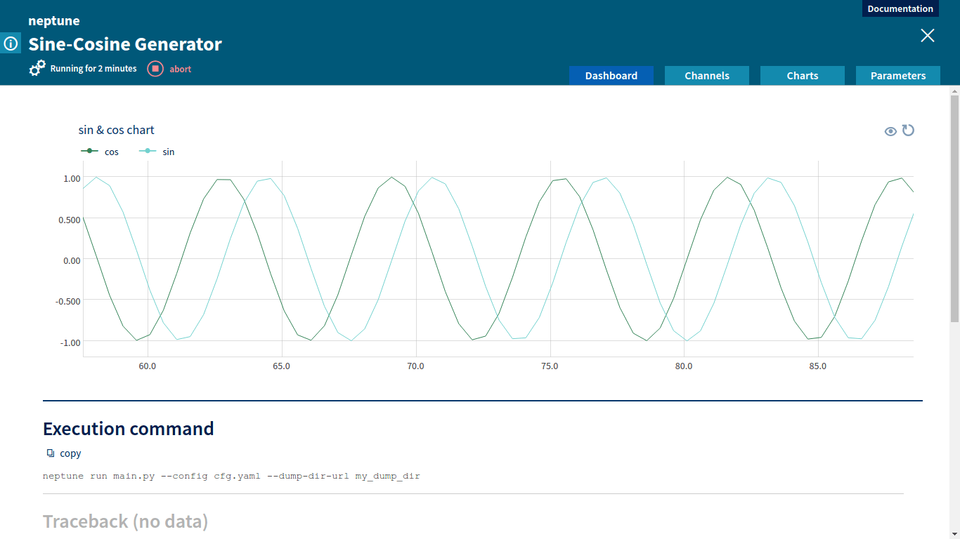
Chart for Sine-Cosine GeneratorCharts displaying custom metrics
For every job a user can define a set of tags. Tags are useful for marking significant differences between jobs and milestones in the project (i.e if we are doing a MINST project, we can start our research by running the job with a well known and publicly available algorithm and tag it ‘benchmark’).
Comparing Results and Collaboration
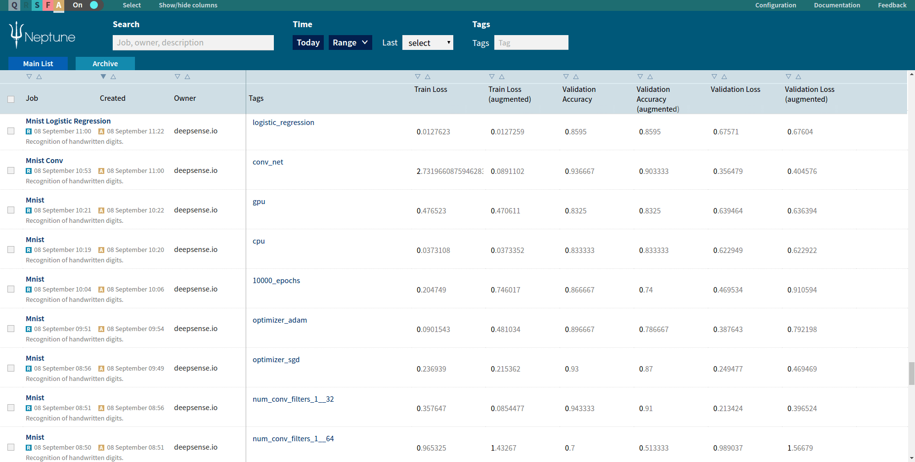
Every job executed in the Neptune machine learning platform is registered and available for browsing. Neptune’s main screen shows a list of all executed jobs. User can filter jobs using job metadata, execution time and tags.
Neptune jobs list
A user can select custom-defined metrics to show as columns on the list. The job list can be sorted using values from every column. That way, a user can select which metric he or she wants to use for comparison, sort all jobs using this metric and then find the job with the best score.
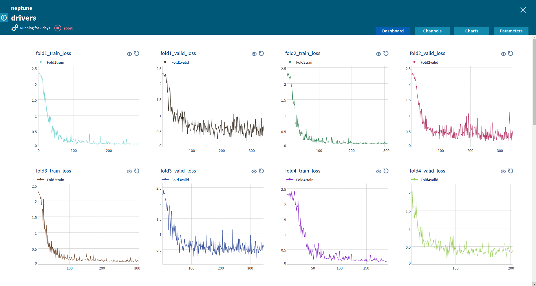
Thanks to a complete history of job executions, data scientists can compare their jobs with jobs executed by their teammates. They can compare results, metrics values, charts and even get access to the snapshot of code of a job they’re interested in.
Thanks to Neptune, the machine learning team at deepsense.ai was able to:
get rid off spreadsheets for keeping history of executed experiments and their metrics values;
eliminate sharing source code across the team as an email attachment or other innovative tricks;
limit communication required to keep track of project progress and achieved milestones;
unify visualisation for metrics and generated data.
In this post, we present new features that come with Seahorse, Release 1.3 – the availability of writing custom operations, data exploration and ad-hoc analysis in R language using Jupyter Notebook. Along with Python (included in the previous Seahorse releases), R is one of the most popular languages in data science. Now, its users can embrace the new release of Seahorse with their favorite R operations included. Spark and R integration is obtained thanks to the SparkR package.
What’s new: R Notebook and custom R operations
There are several ways users can leverage R in their workflows. These include interactive Jupyter R Notebooks, custom R operations for processing data frames and tailor-made R evaluation functions. To demonstrate some of these new features, we are going to work with a dataset regarding credit card clients’ defaults available at the UCI Machine Learning Repository. We will train a model to predict the probability of a default of a loan. The dataset consists of 25 columns and 30K rows. Each row describes a customer of a bank along with information on his/her loan status. The last column – default_payment_next_month is our target variable. For a more detailed description of the dataset, please consult its description page and this paper.
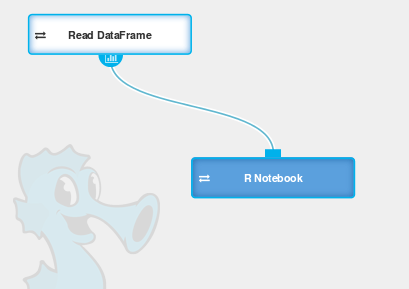
Having loaded the data, we proceed to its initial exploration. To this end, let’s use the R Notebook block from Seahorse’s operations palette.
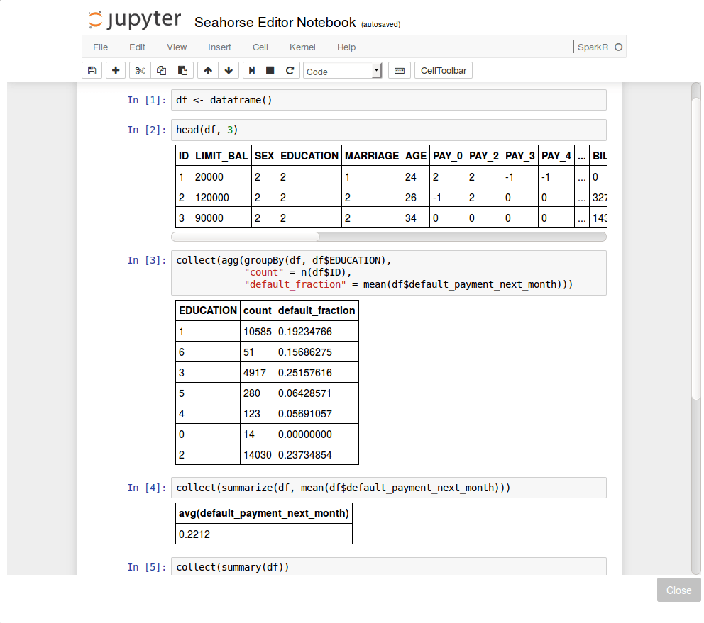
We open the Jupyter Notebook, and start exploring the data. With the use of the dataframe() function we are able to connect to data on the Spark cluster and operate on it. We can invoke it like this: df <- dataframe().
Some of the variables are categorical, for example: Education. In fact, reviewing the dataset documentation, we find that it is an ordinal variable where 0 and 6 denote the lowest and the highest education levels, respectively. In the notebook, after printing out the first three lines of data (the head() command), we performed a sample query for grouping the response variable with respect to education levels and compute the fraction of defaults within the groups. We observe some variability in default fraction with respect to education. Moreover, some of the categories are rare. In total, across all customers, the default fraction is equal about 22%.
Note the use of collect() functions here. This is a Spark-specific operation – it invokes the computation of an appropriate command and returns results to the driver node in a Spark application (in particular, it can be your desktop).
For later analysis we will drop the ID variable as it is irrelevant for prediction. We also see that there are relatively few occurrences of extreme values of the Education variable: 0 and 6 which denote the lowest and highest education levels, respectively. Our decision is to decrease the granularity of this variable and truncate its values to a range of [1, 5]. This can be achieved by a custom R Column Transformation as shown below.
Along with the Education variable, there are also other categorical variables in the dataset such as: marital status or payment statuses. We will not employ any special preprocessing for them since the model that we plan to use – Random Forest – is relatively insensitive to the encoding of categorical variables. Since most of the categories are ordinal, encoding them with consecutive integers is actually a natural choice here. For some other methods, like the logistic regression model, we would need to handle categorical data in a special way, for example, using one-hot-encoder.
To default or not to default
At this point we are ready to train a model. Let’s use the introduced Random Forest classifier, an off-the-shelf ensemble trees machine learning model. We devote 2/3 of data for tuning the model’s parameters – the number of trees in the forest and depth of a single tree – by Grid Search operation available on the palette. The other part of the data will be used for final model evaluation. Since the distribution of the target variable is slightly imbalanced toward “good” labels – about 78% customers in database paid their dues – we will use Area Under ROC as the evaluation metric. This metric is applicable when one class (label) dominates the other. It is more sensitive to retrieval of defaults in data rather than accuracy score (that is, the number of correctly classified instances regardless of their actual class).
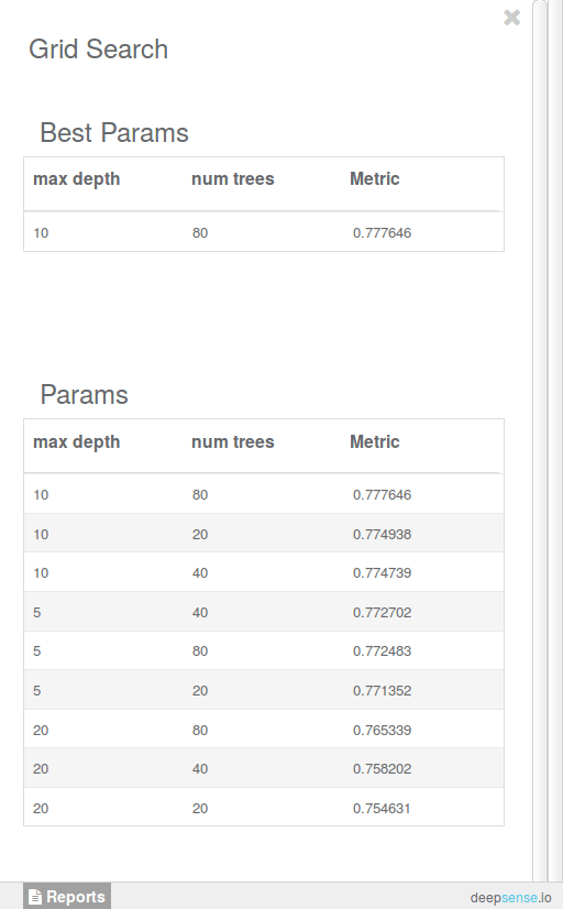
For demonstration purposes, we varied the parameters on a relatively small grid: 20, 40, 80 for the number of trees in the forest and 5, 10, 20 for tree depth. The results of the grid search are presented below:
We see that the optimal values for the number of trees and a tree depth are 80 and 10, respectively. Since there is little difference between choosing 20, 40 or 80 as the number of trees, we will stick with the smallest (and less complex) forest consisting of 20 trees as our final model.
Final check
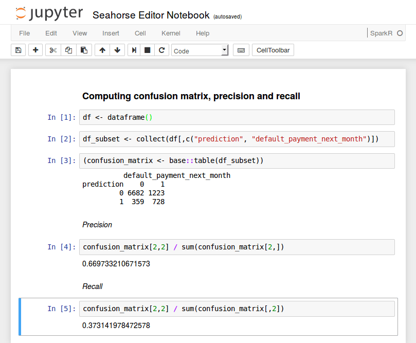
Finally, we evaluate the model on the remaining 1/3 part of data. It achieves a score of 0.7795 AUC on this hold-out dataset. This means that our model learned reasonably well to distinguish between defaulting and non-defaulting customers. For the sake of more interpretable results, the confusion matrix may be helpful. In order to compute it, we will create another R notebook and attach it to the final data with the computed predictions.
The confusion matrix is computed by retrieving two columns from the data frame and aggregating them. This, once again, is done using the collect() function. Here, it fetches the two selected columns to the driver node. Such operations should be performed with care – the result needs to fit into the driver node’s RAM. Here, we only retrieved two columns and there are merely 30K rows in the dataset so the operation succeeds. For larger datasets, we would order the computations to be performed by Spark. Finally, observe that we explicitly called the table() function from R’s base package via base::table(). This is necessary since the R native function is masked once SparkR is loaded.
Let’s proceed to the analysis of the confusion matrix. For example, its bottom left entry denotes that in 359 cases the model falsely predicted default while in fact there wasn’t one. Based on this matrix we may compute the precision and recall statistics. Precision is the fraction of correct predictions (true positives) out of all defaults predicted by our model. Recall is defined as the fraction of correctly predicted defaults divided by the total number of defaults in the data. In our application, precision and recall and equal about 67% and 37%, respectively.
The end
That’s it for today! We presented an analysis of prediction of defaults of a bank’s customers. Throughout the process, we used R for custom operations and exploratory data analysis. We trained the model, optimized and evaluated it. Based on costs associated with customers’ defaults, we can tweak precision and recall by, for example, adjusting the threshold level for probability of the default prediction and the final label (no default vs default) produced by the model. We encourage you to try out your own ideas – the complete workflow is available for download here.
https://deepsense.ai/wp-content/uploads/2019/02/r-notebook-custom-r-operations-new-seahorse-release.jpg217750Jan Lasekhttps://deepsense.ai/wp-content/uploads/2023/10/Logo_black_blue_CLEAN_rgb.pngJan Lasek2016-09-23 08:00:302023-03-06 23:44:58R Notebook and Custom R Operations in the new Seahorse release
deepsense.io is happy to announce a broad cooperation with Open Data Science Conference (ODSC) in London.
deepsense.io’s extensive involvement includes leading the discussion panel on practical machine learning applications (September 21), two workshop sessions (October 1-2), as well as appearance at ODSC UK in London (October 8-9).
During the discussion panel (September 21, 6-9:30 PM, Code Node London), five machine learning data scientists and high level entrepreneurs will gather to discuss the future of machine learning. The panelist list includes Mike MacIntyre (Chief Scientist at Panaseer), Miriam Redi (Research Scientist in the Social Dynamics team at Bell Labs Cambridge), Daniel Hulme (CEO of Satalia), and Jan Milczek (founding member of deepsense.io’s data science team). The discussion will be conducted by Alex Gryn (deepsense.io) and the event will be opened by Jessica Willis (Director of Operations and Business Development, ODSC).
The panelists will talk about possibilities and limitations of machine learning in a variety of industries and science fields, sharing their experience and knowledge. There will also be time for Q&A session. The event is fully booked (300 RVSP with the waiting list open). Please find more details, including the agenda at meetup.com.
Learn the latest models, advancements and trends from Machine Learning and Deep Learning creators and top practitioners at the MLDL Conference at ODSC UK 2016. Learn more at odsc.com.
As a part of the ODSC UK 2016 Introductory Workshops series, deepsense.io will provide two workshops for beginners (General Assembly London), run by Jan Lasek and Julian Zubek. The first session, Intro to Machine Learning (October 1), will cover an overview of the machine learning ecosystem with an emphasis on actual case studies across various industries. To provide more context, the session will start with a gentle theoretical outline and smoothly dive into selected concepts. On October 2, deepsense.io’s instructors will conduct Intro to Data Science with Python – hands-on training for programmers. Both sessions are open for registration for all ODSC UK 2016 ticket holders. The number of seats is limited. Additional information is available at odsc.com.
deepsense.io is also proud to support ODSC UK 2016 as a Gold Sponsor. On October 8 and 9, conference participants will have an opportunity to try our newest platform for efficient management and monitoring of machine learning experiments, Neptune. Mariusz Gadarowski, Neptune’s Product Director, will deliver a session about challenges in data science processes and introduce Neptune as a solution.
The conference takes place at Hotel Novotel London West. Tickets are available at odsc.com. Use discount code: ODSC-DEEPSENSE for an additional 40% Off tickets to ODSC UK 2016.
###
About deepsense.ai:
Media contact:
deepsense.ai trademarks at boilerplate
https://deepsense.ai/wp-content/uploads/2019/02/odsc-uk-2016-open-data-science-conference-and-deepsense-io-take-londons-machine-learning-scene-by-storm.jpg3371140Barbara Rutkowskahttps://deepsense.ai/wp-content/uploads/2023/10/Logo_black_blue_CLEAN_rgb.pngBarbara Rutkowska2016-09-21 12:01:282022-12-02 17:43:18ODSC UK 2016: Open Data Science Conference and deepsense.io Take London’s Machine Learning Scene By Storm