Driverless car or autonomous driving? Tackling the challenges of autonomous vehicles
Among both traditional carmakers and cutting-edge tech behemoths, there is massive competition to bring autonomous vehicles to market.
It was a beautiful, sunny day of June 18, 1914 when the brilliant engineer Lawrence Sperry stunned the jury of Concours de la Securité en Aéroplane (Airline Safety Competition) by flying in front of their lodge with his hands held high. It was the first time the public had ever seen a gyroscopic stabilizer, one of the first autopiloting devices. Over a hundred years later, automatic flight control devices and maritime autopilots are common, while cars still require human operation. Thanks to machine learning and autonomous cars, that’s about to change.
What is the future of autonomous vehicles?
According to recent reports, autonomous cars are going to disrupt the private, public and freight transportation industries. A recent Deloitte publication reports that society is putting more and more trust in autonomous vehicles. In 2017, 74% of US, 72% of German and 69% of Canadian respondents declared that fully autonomous cars would not be safe. But those rates have now dropped significantly, to 47%, 45% and 44%, respectively.
Plans for building self-driving cars have been revealed by BMW, Nissan and Ford, while Uber and the Google-affiliated Waymo are also in the thick of the race. Companies aim both to build urban driving vehicles and autonomous trucks, while a startup scene supporting autonomous technology is emerging.
Thanks to the increasing popularity of autonomous cars, up to 40% of mileage could be driven in self-driving vehicles in 2030. But, as always, the devil is in the details.
What is an autonomous car?
To answer that question, the National Highway Traffic Safety Administration uses the autonomous vehicle taxonomy designed by the Society of Automotive Engineers, which lists five levels of automation.
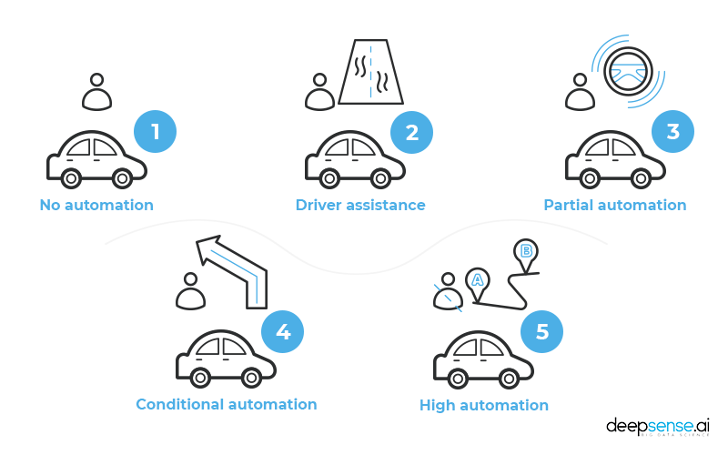
- No automation – the driver performs all driving tasks
- Driver assistance – the car has built-in functions to assist the driver, who nonetheless must remain engaged in the driving process. Cruise control is one of the best examples.
- Partial automation – the vehicle has combined automated functions like acceleration and steering, but the driver must remain engaged. The gyroscopic stabilizer is an example of partial automation.
- Conditional automation – a human driver is necessary in totally unpredictable situations, but not required to monitor the environment all the time. BMW currently has a fleet of about 40 level 4 cars unleashed on testing grounds near Munich and in California.
- High automation – the car on this level may not even have a steering wheel and can deal with any situation encountered. Fully autonomous vehicles, which do not yet exist, occupy Level 5.
Building level 4 and 5 driverless vehicles is a great challenge because the driving process has a number of complicating factors. Unlike with a plane or ship, drivers usually have little to no time to respond to the changing environment. They must monitor the state of the machine, their surroundings, and the other drivers on the road. What’s more, any mistake can cause an accident – 37.133 people were killed in traffic accidents on American roads in 2017.
While we may not give ourselves credit as drivers, humans’ ability to process signals from various senses to control a car is a super power. It is not only about simply looking at the road – many drivers estimate the distance between cars by looking at reflections in the body of the car in front of it. Many drivers can hear changes in their engine’s performance or sense changing grip strength on various types of road.
To effectively replace human perception, sophisticated assistance systems rely on numerous sensors. GM’s report on autonomous cars and driving technology safety lists:
- Cameras – detect and track pedestrians and cyclists, monitor free space and traffic lights
- Articulating radars – detect moving vehicles at long range over a wide field of view
- Short-range radars – monitor objects around the vehicle
- Long-range radars – detect vehicles and measure velocity
- Lidars – detect fixed and moving with objects high-precision laser sensors
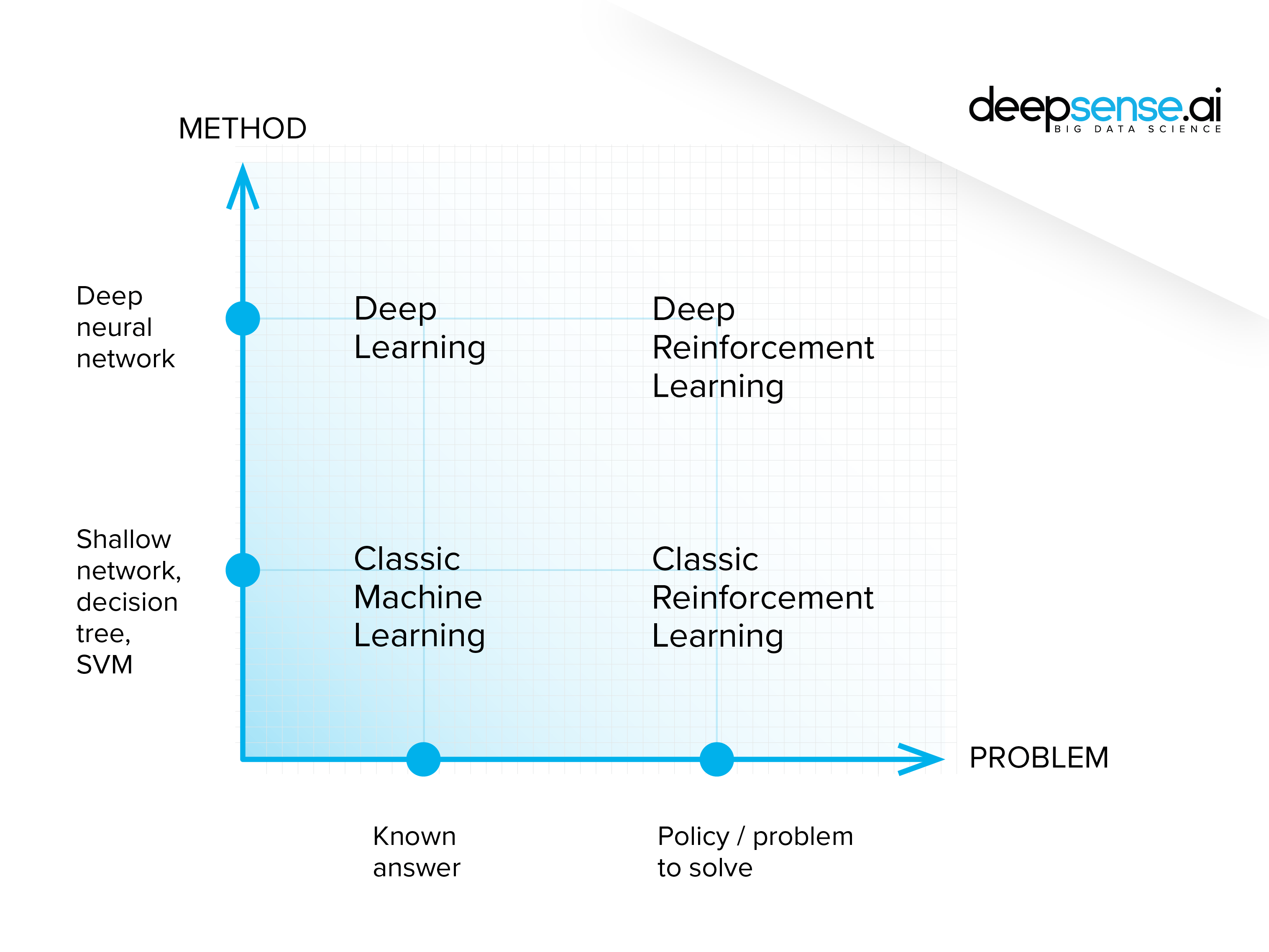
Handling data from various sources that need to be processed in real time is a perfect task for deep neural networks, especially when it involves simultaneous work on non homogenous data taken from radars, images from cameras and lidar readings.
But building a system that automates driving is an enormous challenge, especially given the sheer number of serious decisions to be made when driving and the fact that a single bad decision can result in disaster.
Two ways how autonomous cars work
There are currently two approaches to building the models that control autonomous vehicles.
A component-based system – the controller is built with several independent models and software components each designed to handle one task, be it road sign recognition, managing the state of the vehicle or interpreting the sensors’ signals.
- Pros – dividing the system into subsystems makes building the software easier. Each component can be optimized and developed individually thus improving the system as a whole.
- Cons – developing the model requires a massive amount of data to be gathered and processed. The image recognition module needs to be fed different data than the engine control device. This makes preparing the dataset to train more than a little challenging. What’s more, the process of integrating the subsystems may be a challenge in and of itself.
End-to-end system – with this approach, a single model capable of conducting the entire driving process is built – from gathering information from the sensors to steering and reacting accordingly. deepsense.ai is moving ahead with just such a model.
- Pros – it is easier to perform all the training within the simulation environment. Modern simulators provide the model with a high-quality, diverse urban environment. Using the simulated environment greatly reduces the cost of gathering data.
Although it is possible to label and prepare data gathered with the simulator, the technique requires a bit more effort. What’s more, it is possible to use a pre-trained neural network to mimic the simulated environment (a matrix of sorts) to further reduce the data to gather or generate. We expect the model to perform better than a component-based system would.
- Cons – this type of model may be harder to interpret or reverse-engineer. When it comes to further tuning the model or reducing the challenge posed by the reality gap (see below) it may be a significant obstacle.
Facing the reality gap
Using a simulator-trained model in a real car is always challenging due to what is known as the reality gap. The reality gap represents all the differences and unexpected situations the model may encounter than the designer was able to predict and therefore prepare it for.
There are countless examples. The position of cameras in a real car may be different than in a simulated one, the simulation physics are necessarily incomplete, and there may be a hidden bug the model could exploit. Furthermore, the sensors’ readings may differ from the real ones concerning calibration or precision. There may be a construction feature that causes the car to behave differently in reality than in a simulation. Even the brightest data scientist is unable to predict all the possible scenarios. What would happen if a bird started to peck at the camera? Or if a car encountered a boy dressed as Superman pretending to fly? Or, more plausibly, after a collision, if there were an oil stain that looked exactly like a puddle, but would obviously have an entirely different effect on the tires’ grip of the road?
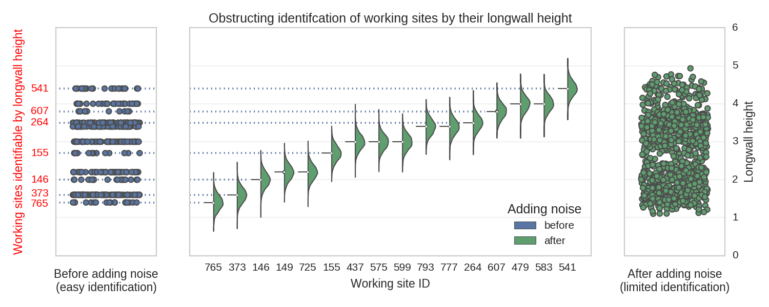
To address these challenges, data scientists randomize the data and the training environment to let the model gather more varied experiences. The model will learn how to control the car in changing weather and lighting conditions. By changing the camera and sensor settings, a neural network will gain enough experience to handle the differences or any changes that may occur when the model is being used.
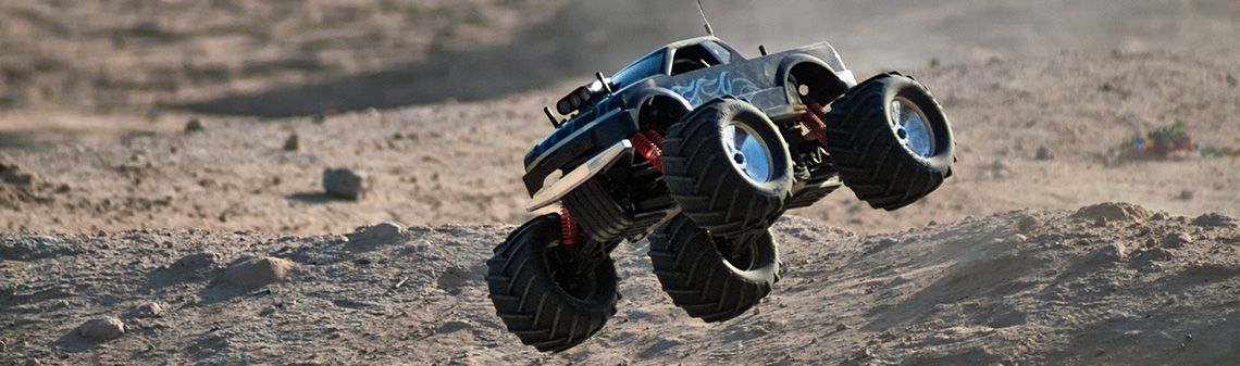
Fighting the gap every lap
Using a simulated environment is one effective way of evaluating a model, but a pronounced reality gap still remains. To acquire better information (and also to have some fun on the job), data scientists evaluate their neural networks by launching them in small-scale models. There is currently an interesting Formula 1/10 autonomous car racing competition being held. Designing the software to control cars and compete against other teams is a challenging (yet fun) way to evaluate models. Small-scale models are tested on tracks with angles and long straights that are perfect for acceleration. Although the cars aren’t driven by humans, the team provides full-time technical assistance and puts the car back on track when it falters.
It’s also a great way to impress the jury in a similar manner to what Lawrence Sperry did more than a hundred years ago!
If this sounds interesting to you, deepsense.ai has recently launched a deep learning workshop where participants will learn to create models to control these small cars. The training will be conducted in cooperation with one of world champion Formula 1/10 racers.
The text was prepared in cooperation with Krzysztof Galias, deepsense.ai data scientist.