Diffusion models in practice. Part 2: How good is your model?

This is the second post in our series “Diffusion models in practice”. In this article, we start our journey into the practical aspects of diffusion modeling, which we found even more exciting. First, we would like to address a fundamental question that arises when one begins to venture into the realm of generative models: Where to start?

Introduction

This is the second post in our series “Diffusion models in practice”. In the previous one, we established a strong theoretical background for the rest of the series. We talked about diffusion in deep learning, models that utilize it to generate images, and several ways of fine-tuning it to customize your generative model. We also explained the building blocks of Stable Diffusion and highlighted why its release last year was such a groundbreaking achievement. If you haven’t read it before, we strongly recommend you start there [1]!

In this post, we start our journey into the practical aspects of diffusion modeling, which we found even more exciting. First, we would like to address a fundamental question that arises when one begins to venture into the realm of generative models: Where to start?

So many options…

Both the rapid ongoing development and the lack of general know-how in the scope of diffusion models and surrounding techniques results in many people getting confused even before they begin.

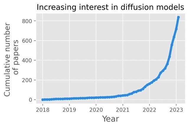
In the previous post, we explained the importance of Stable Diffusion [3]. The Hugging Face hub [4] already contains hundreds of models with unique adaptations. There are also numerous techniques used to fine-tune the model (which we covered in the last post) – each yielding satisfactory results. On top of that, the models can be used for a variety of different tasks revolving around image generation, such as inpainting, outpainting, image mixing, using smart starting noises, and many more.

Being spoiled for choice is usually a good thing, but keeping up is quite problematic – before you fine-tune your favorite new model, there is another state-of-the-art solution waiting to be explored. Important choices not only refer to the abstract topic of architecture. After selecting your weapon of choice, another rabbit hole opens up: parametrization. Each of the models and methods comes with dozens of parameters for both training and generation, with an exponential number of combinations. Both inherent variance in output quality and the lack of fixed criteria of what constitutes good results make the search for perfect parameters truly challenging.

All of that can leave even the toughest deep-learning practitioner confused. But don’t worry! In this and future posts, we would like to explain our empirical and data-based approach to enable rational assessment and choices. These helped us navigate the complications and we hope that it will be beneficial for others as well. Let’s dive into it!

How can we estimate fine-tuning quality? 

Let’s assume that we managed to choose our favorite model. More than that, we adapted it to our needs via fine-tuning. That’s great news! But how can we assess the quality of our adjustments? The visual inspection always comes first, but when done ad-hoc it’s by no means informative nor reproducible. We would like to have a solution that is as automatic as possible, as well as being reliable.

Several natural metrics immediately come to mind, one of which makes it possible to establish how similar the output of our model is to the object that we embedded in the model domain during fine-tuning. Another can inform the user about the aesthetic value of the image. So how can we actually measure those? We decided to use the human-like approach i.e. look at the input/output images and estimate the performance of the model using subjective criteria. The metrics described below were proposed and validated based on one specific type of object: faces.

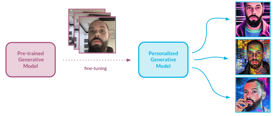
However, with small adjustments, the approach we describe below can be applied to any domain. Most importantly, the general methodology for the validation can be used for any generative setup.

Similarity assessment

Our goal is to gather insights into how well the model understands the images that were provided during the training, or in our case, fine-tuning. The similarity of object’s characteristics between real picture and the output is vital for a high-quality model. To make sure the model has acquired knowledge about the characteristics of new objects, there is a need for a validation setup that provides information about how similar the object is to the generated image when compared to the dataset used for fine-tuning.

Usually, we would like the model to generate our object in different setups, styles, and scenarios. A different textual input prompt means different colors and textures in the images. What we truly care about is how well our model conveys the characteristics of the object to an image.

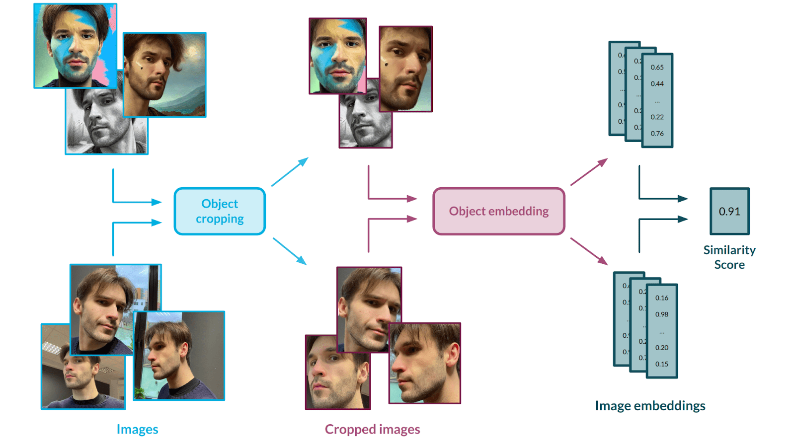
To measure that, we use a two-stage solution – first, we crop out the object from pictures, as this is the only part we want to measure the similarity for. Next, we embed the images using an Inception-based [5] neural network. Let’s talk about those models and the validation scheme we used to make sure they are the right fit for our approach.

Face cropping

We opted for the MTCNN [6] architecture which is specifically trained for the task of face cropping, but a similar architecture can be applied to any other type of object. This solution is based on several Convolutional Neural Networks that work in a cascade fashion to locate the face with some landmarks in an image.

The first network is called a Proposal Network – it parses the image and selects several bounding boxes that surround an object of interest: a face, in our case. It is the fastest of all three networks since its main job is to perform basic filtering and produce a number of candidate boxes. In the second step, the candidates are fed into a Refine Network, which further reduces the number of false candidates and refines the bounding box locations. The third and last network, the Output Network, performs the final adjustments and additionally provides information about facial landmarks. In this model, the location of 5 landmarks is predicted – the left and right eyes, the left and right corners of the mouth, and the nose.

Architecture links several tasks of different natures. One is a face classification, where a classical cross-entropy loss is used. The others are bounding box regression and facial landmark localization, where updated weights are calculated via Euclidean loss functions. Each network’s prediction finishes with a non-maximum suppression mechanism to merge lots of boxes into the most likely candidates.

Needless to say, other tools can be applied with similar effects here, including architectures that are not designed to work with facial images.

Face embedding

Having extracted the faces, we opted for InceptionResnetV1 [8] as an encoder to allow for reliable comparison. This model can boil the input down to a numerical representation, which allows it to represent the abstract images in a pleasant, vector form. It was originally trained on the VGGFace2 [9] dataset containing 3.31 million images across over 9000 identities. In the case of other objects, other versions of the Inception-based network could be used.

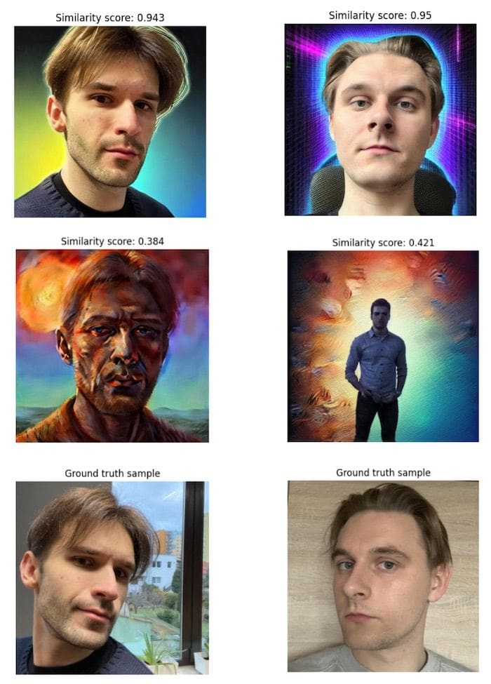
To assess how similar the faces in two images are to each other, we simply run the generated images through the model together with the input image and we receive vector embeddings. This allows us to run any type of statistical analysis on the vectors – we opted for cosine similarity. The score is a mean aggregation of every generated image versus input similarity, which allows us to achieve a statistically relevant outcome.

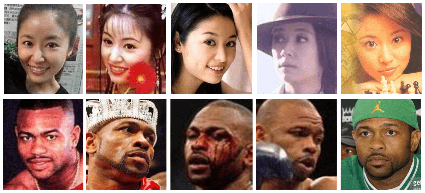
How does it work? InceptionResnetV1, trained beforehand on a significant number of different faces, can extract their features and encode their representations in a way that the similar faces are represented through vectors that lie close together in vector space.

Aesthetic assessment

Aesthetic measurement is a second important metric that helps to establish how powerful a model is. Image aesthetics is a pretty abstract concept, which is difficult to grasp and define even for a human. Strictly defining it with mathematical formulas could prove impossible; hence, we decided to model it using data. For that purpose, we used a publicly available dataset with subjective aesthetic assessments gathered from people. To best represent the images, we decided on the CLIP [10] model from OpenAI – the same architecture that is used in the Stable Diffusion [3] pipeline. CLIP works as a well-defined mapping between images and text – we covered it in a previous post in this series [1].

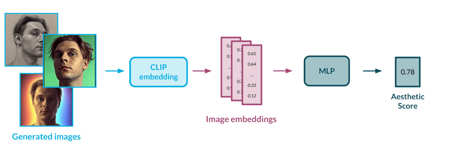
Having a way to represent images in numerical form, there was a need to automate the process of evaluating the aesthetics of a given image. To do this, we used an AVA dataset [11] containing more than 250,000 images, along with assessments of their aesthetics by various people. Our goal was to train a multi-layer neural network in a regression setup to teach it the abstract correlation between face characteristics and aesthetic value. The model would rate each image on a scale from 0 (poor aesthetics) to 10 (great aesthetics). We applied data balancing methods to the input dataset to influence the rating distribution, as the first model’s outputs were highly condensed in the middle of the scale – the model had problems estimating extreme values, e.g., 1-2 or 9-10.

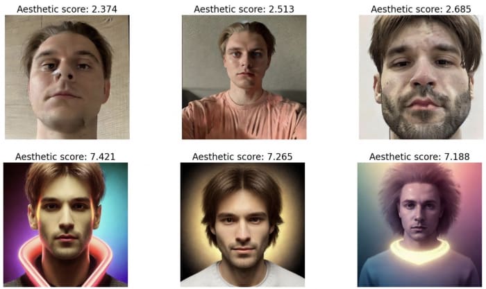
It is worth noting that the LAION dataset [12] on which Stable Diffusion was trained also has aesthetic evaluations. While it might have been easier to use that one, it could lead to unwanted data leakage, which is why we depended on an external dataset.

Metrics in action

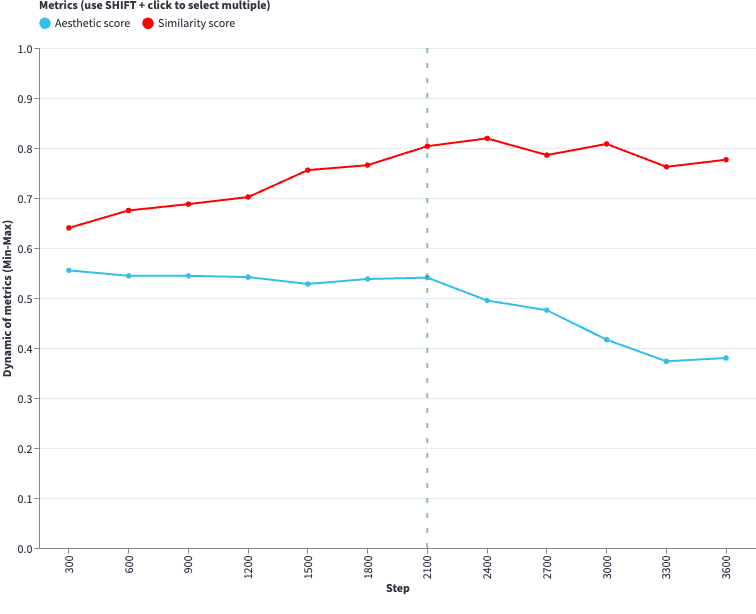
Enough talk! That was a comprehensive description of the metrics – it is time to see how they work. Let’s ask ourselves one of the many valid questions we might have when thinking about model fine-tuning – how many input images do I need to use?

The graph above should help you find the answer to that question. It is fully interactive, so feel free to explore it. We fine-tuned the Stable Diffusion v1.5 model on pictures of several people, and tested a different number of input images to see how it affects the training of the model. You can trace how different metrics behave during the evaluation every 300 steps and how it affects the images produced.

Visual inspection allowed us to notice that the presented metrics work well, scoring comparably to humans. However, we would not feel comfortable without validating those setups, so we decided to make sure we can rely on them to provide us with accurate information. We strongly recommend you visit Appendix A to see exactly how it was done!

Summary

In this post, we expressed how confusing it might be to successfully navigate the convoluted area of diffusion models, in both a theoretical and practical sense. To make matters simpler, we introduced two metrics that come in very handy when a reliable assessment of the models is needed. We proved that these models are well-balanced and suitable for our needs with comprehensive validation. In the next post of this series, we will expand on this approach, with lots of experiments and more metrics to check them. Stay tuned!

Appendix A – Metrics validation

For validation purposes, we used images of 8 different people – 4 women and 4 men – to fine-tune 8 new v1.5 Stable Diffusion models. We used the same number of images to fine-tune the models for all of the subjects. After training, two evaluation datasets were created by generating 128 pictures with each model, using half of the images for similarity validation and the other half for aesthetic validation.

Five different people marked the aforementioned sets of pictures according to their subjective opinion. Each image received a label from 1 to 5 (Likert scale [13]) from each labeler, with one meaning very bad and five being very good. This type of labeling was done for both metrics separately. After that, we could calculate several statistics, such as each evaluator’s grade, which is essentially a mathematical formulation of how the given labeler assesses the images. For all of the proper definitions, please check out Appendix B of this post.

Every set was then divided into 5 cross-validation sets in a 4:1 ratio considering the labeler’s dimension – in each set, the labels from one labeler were included in the test set. Using our proposed evaluation as the function we want to optimize, we undertook model score mapping (bucket division) on a scale of 1 to 5 on the validation sets. We performed the bucketizing in a way that minimizes the distance between the model and human answers.

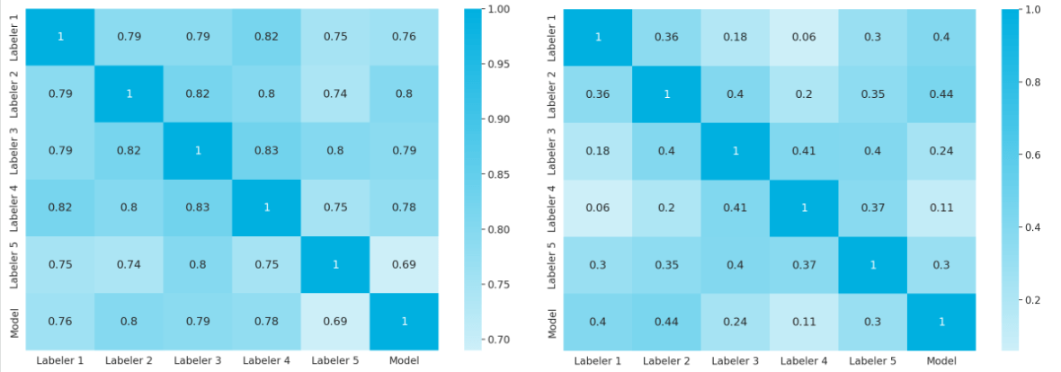
Next, we tested the model score (similar to the test set labeler) and averaged it out over 5 test sets. We can observe that there is a highly positive correlation between human labels and the score predicted by the similarity model.

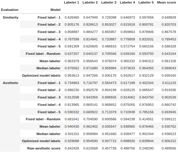
In the table below we present the results of cross-validation of the model. After optimization, the models perform in a human-like fashion – exactly what we aimed for!

Appendix B

Let’s denote \(E\) as the set of evaluators of a given set of images \(S\). We can formulate a discrete Likert scale evaluation as

$$
\begin{equation}
\forall e \in E \;\; \forall s \in S \quad e_d(s) \in L.
\end{equation}
$$

Each score is normalized so that the scores are within the \([0, 1]\) interval, which we can describe as a scoring function \(e\):

\begin{equation}
\forall e \in E \;\; \forall s \in S \quad e(s) \in [0,1].
\end{equation}

For each evaluator, we can define a mean evaluator score on the set of images \(S\) as

\begin{equation}
\forall e \in E \quad \bar{e}=\dfrac{\sum\limits_{s \in S} e(s)}{|S|}
\end{equation}

as well as the standard deviation of the evaluator score on the set of images S

\begin{equation}
\forall e \in E \quad \sigma(e)=\sqrt{\dfrac{\sum\limits_{s \in S}(e(s)-\bar{e})^{2}}{|S|}},
\end{equation}

where \(|S|\) denotes the cardinality of the set of images.

For a single image sample, we can define a sample score \(\bar{s}\) as
\begin{equation}
\forall s \in S \quad \bar{s}=\dfrac{\sum\limits_{e \in E} e(s)}{|E|}.
\end{equation}

Specifically for the single evaluator grading, we include a modification of the above score \(s\) established for each labeler. Let’s denote \(E_{e}\) as the set of evaluators without evaluator \(e(\forall e \in E \; E_{e} = E\setminus{e})\). We can define a sample score without the evaluator \(e\) as:
\begin{equation}
\forall e \in E \;\; \forall s \in S \quad \bar{s}_e=\dfrac{\sum\limits_{e \in E_e} e(s)}{\left|E_e\right|}.
\end{equation}
For a single evaluator \(e\) we can define his grade on the set of images \(S\), denoted as \(g(e)\), which is referred to as evaluator’s grade
\begin{equation}
\forall e \in E \quad g(e)=1-\frac{\sum\limits_{s \in S}\left|e(s)-\bar{s}_e\right|^k}{|S|},
\end{equation}

where \(k \in \mathbb{N}+\) is a grading parameter.

References

1. https://deepsense.ai/diffusion-models-in-practice-part-1-the-tools-of-the-trade/
2. https://vsehwag.github.io/blog/2023/2/all_papers_on_diffusion.html
3. High-Resolution Image Synthesis with Latent Diffusion Models, Rombach et al. 2022
4. https://huggingface.co/models?other=stable-diffusion
5. Going deeper with convolutions, Szegedy et al. 2014
6. Joint Face Detection and Alignment Using Multitask Cascaded Convolutional Networks, Zhang et al. 2016
7. https://kpzhang93.github.io/MTCNN_face_detection_alignment/index.html
8. Inception-v4, Inception-ResNet and the Impact of Residual Connections on Learning, Szegedy et al. 2016
9. VGGFace2: A dataset for recognising faces across pose and age, Cao et al. 2018
10. Learning Transferable Visual Models From Natural Language Supervision, Radford et al. 2021
11. AVA: A Large-Scale Database for Aesthetic Visual Analysis, Naila Murray and Luca Marchesotti and Florent Perronnin, 2012
12. https://laion.ai/blog/laion-5b/
13. https://simplypsychology.org/likert-scale.html