Table of contents
In previous blog posts, we introduced you to the world of diffusion models. We also proposed an evaluation method for various aspects of generative models based on the example domain of face generation. We now use the previously introduced metrics imitating human-like assessment.
Table of contents
- Introduction
- Experimental setup
- Questions and empirical answers
- Summary
- Appendix – Diversity calculation
Introduction
In previous blog posts, we introduced you to the world of diffusion models. We also proposed an evaluation method for various aspects of generative models based on the example domain of face generation. We now use the previously introduced metrics imitating human-like assessment. By combining theoretical concepts and empirical experimentation, we aim to provide comprehensive and evidence-based answers to the hidden questions that often arise in the fine-tuning of these models. The specific domain we have selected is personalized face image generation, but the conclusions and methodology are applicable elsewhere as well. So get ready to explore the world of stable diffusion from a unique perspective as we share our insights and findings using the methods we’ve developed!
What are we trying to achieve?
It is essential to grasp the core of our research before moving forward. Here, we provide a condensed glimpse into our objectives, the data we analyze, our approach to prompt engineering, and the computational power propelling our discoveries.
The generation of a specific class of images using diffusion models capable of a broader range of expressions is a common scenario. To reflect this, we chose the generation of personalized 512×512 images of faces as a particular subdomain. The aim here is to optimize:
- the ratio of the images staying within the selected domain (i.e. portraits),
- the visual appeal of the images,
- the similarity to the person specified,
- the diversity of the outputs.
With those goals in mind, we wish to provide some answers to the following questions:
- What does the dynamic of fine-tuning look like?
- How long should the model be tuned?
- How many images should be used for satisfactory results?
- Which prompts are good?
- Do the popular negative prompts affect the generation?
Experimental setup
In this subsection, we will peel back the curtain and reveal the essential components of our experiments. We will provide an in-depth look at the data we employed, the hardware that powered our endeavors, the intricacies of prompt engineering, and the metrics used to evaluate the performance of the model.
Data – the fuel of our experiments
While diffusion models can generate practically any image, one is usually interested in a specific domain with intrinsic quality criteria. As an example domain in which to test our empirical methods, we chose personalized portrait generation. The choice was a very conscious one. Portrait generation is popular; quality assessment is intuitive and requires no experience; several partial, domain-specific metrics are easy to conceptualize (similarity to a given person, aesthetic quality, etc.); and the conclusions may translate well to other domains.
To hone in on the intricacies of diffusion model-based facial image generation, we created a photo portrait input dataset including:
- 10 different people (five women, five men)
- 28 high-quality images per person
- various expressions, angles, and details per person
This selection ensured relative diversity and representativeness. Based on this, portrait generation proved a fruitful environment for investigating the capabilities of diffusion models in terms of generating realistic and diverse samples, allowing us to shed some light on the general properties of diffusion models.
The computing power
Now, a few words about the hardware that allowed us to breathe some life into our models and data, and to perform the experiments.
Stable Diffusion, in its basic form, requires about 40 GB of VRAM to train. With some optimizations, the most ‘inclusive’ setup on which we run DreamBooth finetuning was RTX 2080 Ti, with 12GB of VRAM. We utilized four such GPUs.
We took advantage of various optimizations to achieve this. They included an 8-bit Adam optimizer, gradient checkpointing, and caching images already embedded in latent space. These optimizations helped us manage memory usage effectively, enabling us to work around the limitations.
Prompt-crafting
Prompt engineering is a crucial aspect of our experiments, as it sets the stage for generating meaningful outputs from diffusion.

We used this template to generate a diverse and robust set of 5000 prompts by randomly replacing prompt components with their corresponding values (see table below). The word “customcls” contained in the template is a token of the object we fine-tune for, while CLASS TOKEN is the ‘base object’, i.e. a similar object already present in the domain before fine-tuning (in our, either “man” or “woman”).
We utilized these 5000 prompts during the inference experiments to generate images and assess the performance of any diffusion model. In the training validation process, we carefully selected a subset of 100 prompts and used it at intervals during the training procedures. This allowed us to craft representative input sets and achieve controlled, interpretable results within a reasonable timeframe.
Evaluation metrics
Evaluation metrics are a critical but problematic element of generative model assessment. In our previous blog post, we introduced and evaluated similarity and aesthetics metrics. We encourage you to check it out in detail. In addition to these two metrics, there is another crucial indicator of model quality, namely output diversity.
In the literature, the FID Score is often used for similar purposes, as a state-of-the-art method. Simply put, the FID Score assumes that the model’s training dataset and output set are normal distributions and measures the distance between them. We opted to modify this approach slightly, as we are only interested in the diversity of the model’s generation after fine-tuning, not its comparisons with either the (tiny) fine-tuning or (huge) pre-training dataset. Our diversity assessment directly measures variation in the generated image sets during evaluation. When tracking diversity, we want to ensure that the variety of images produced by the model does not decrease significantly from the base value at the starting point. A detailed description of how we calculate the output diversity is described in the Appendix.
By measuring the metric dynamics during the training, we can track the model’s performance and check that the quality of the generated images does not degrade over time.
After we calculated all the metrics for all the relevant images, we scaled them to ranges allowing for the best presentation of the differences that occurred. The assumed min-max metric value ranges are:
- 0.45 – 0.85 for similarity
- 0.3 – 0.7 for aesthetics
- 0.5 – 0.75 for diversity
Questions and empirical answers
Having discussed the technicalities, we can address some of the most pressing questions related to the parametrization of diffusion models and provide answers backed by data and empirical analysis.
We decided to present our observations accompanied by fully interactive graphs to allow the reader to explore the data and draw his own conclusions.
Our data presentation follows our experimental method, and includes these steps:
- Selection of the independent variable to be studied (training steps, input image count, etc.),
- Preparation of mass training or inference processes, exploring the space of the variable in question on all subjects (individuals) within the dataset,
- Generation of the images from a previously described set of prompts (100 for training experiments and 5,000 for inference experiments),
- Evaluation of all the generated images in terms of the assumed metrics,
- Conducting visual analysis.
How do the metrics change during fine-tuning?
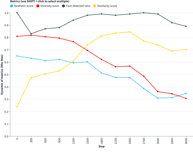
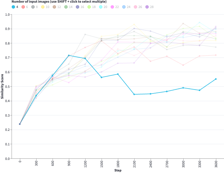
The first chart shows the dynamics of fine-tuning runs. Based on the metric changes, one can make a number of hypotheses and observations:
- Training tends to follow a trend: gradual improvement followed by a collapse in quality.
- The number of input images prolongs the process in a near-linear fashion: the more images, the slower the training/collapse.
- The similarity score monotonically increases almost until the end, even well into the collapse.
- Most of the time, the aesthetic score monotonically decreases. Manual checks confirm that dramatic drops in the aesthetic score indicate training degeneration in the form of artifacts in the generated images.
- Diversity monotonically decreases. Again, significant drops indicate overfitting and an associated collapse in quality.
- Gender bias exists:
- Females tend to produce more attractive photos (obviously).
- Higher similarity values are easier to achieve for males.
https://diffusion-charts.deepsense.ai/post03_chart001
Caption: Metrics dynamics during training process.
So when should I stop training my model?
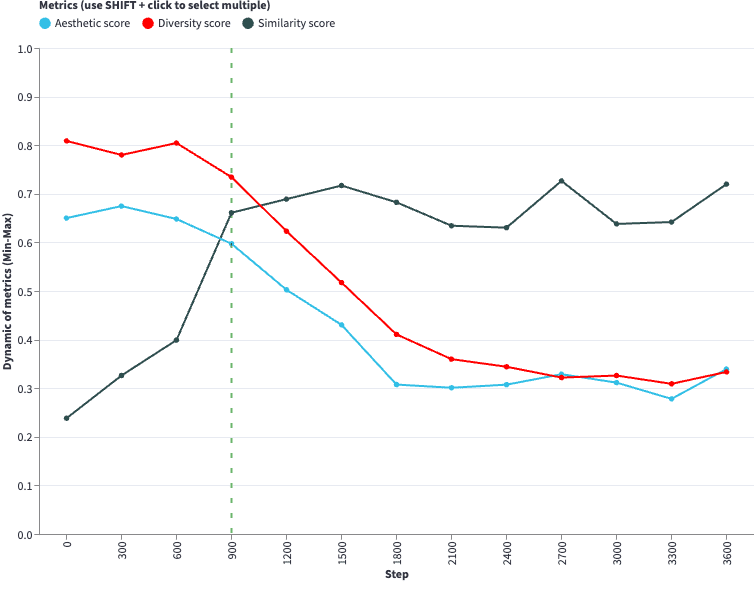
If the metrics can signal the breaking point in training, it may be a good sign that it’s time to stop. Since we monitor multiple competing performance dimensions (metrics), different tradeoffs between similarity, aesthetics, and diversity are possible. To accommodate this, we provided weights for each metric. You can use it to adjust the optimal/stop points to your preferences (we used our preferred weights as a starting point).
This way, we can also verify various popular rules of thumb. One well-known heuristic states that the optimal number of steps is 100 * the number of input images. It seems close to the truth, but other options may possibly work better (note that values may change slightly for your metric weights):
- for males: 120 * the number of input images
- for females: 150 * the number of input images
https://diffusion-charts.deepsense.ai/post03_chart003
Caption: Dynamics of specific metrics for different fine-tuning dataset size.
What’s the impact of changing the number of input images? What number of input images is sufficient?
Let’s try to use this approach to answer another question that has long troubled the community involved in generative art: what is the influence of the number of input images on the quality of the output?
- The optimal training length is closely related to the input image count. The more input images we use for fine-tuning, the longer it will take to reach the maximum similarity value and the minimum aesthetic and diversity values.
- Could we see more if we presented the data some other way?
https://diffusion-charts.deepsense.ai/post03_chart002
Caption: Optimal early-stopping moment based on the dynamics of specific training runs.
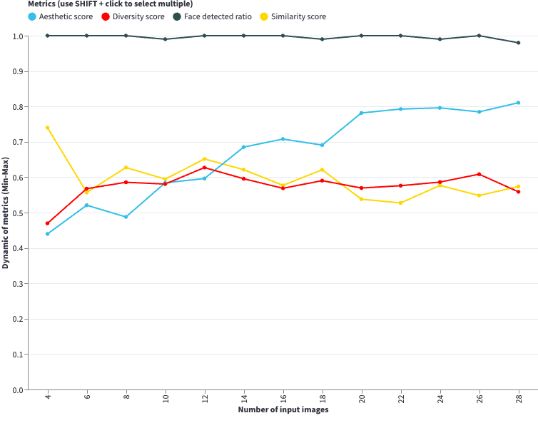
Instead of focusing on the training dynamics, the graph below inspects a direct relationship between the number of images and the metric values at the final/optimal point of the training. We can see that:
- Indeed the similarity seems optimal with a dataset consisting of 12/14 images. However, the increasing number of source images may influence the similarity metrics itself (e.g. it is easier to overfit to 12 images than to 24), so one needs to be careful not to reach too far when drawing conclusions in this case, especially considering the next point.
- The final aesthetics and diversity of images produced grow with the number of images. In our interpretation, even 12 images can produce decent results, but for optimal quality one may want to use as many as 20+ images, despite the questionable indication of the loss of similarity.
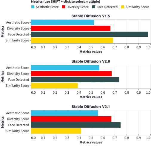
- The 2.0 and 2.1 versions of the model perform significantly worse than the 1.5 model based on which we presented the earlier results. We will inspect this issue more closely now.
https://diffusion-charts.deepsense.ai/post03_chart004
Caption: Mean metrics values in optimal early-stopping moments for different image numbers.
Model comparison
It is no surprise that Stable Diffusion versions 2.0 and 2.1 are capable of significantly better generation than 1.5.
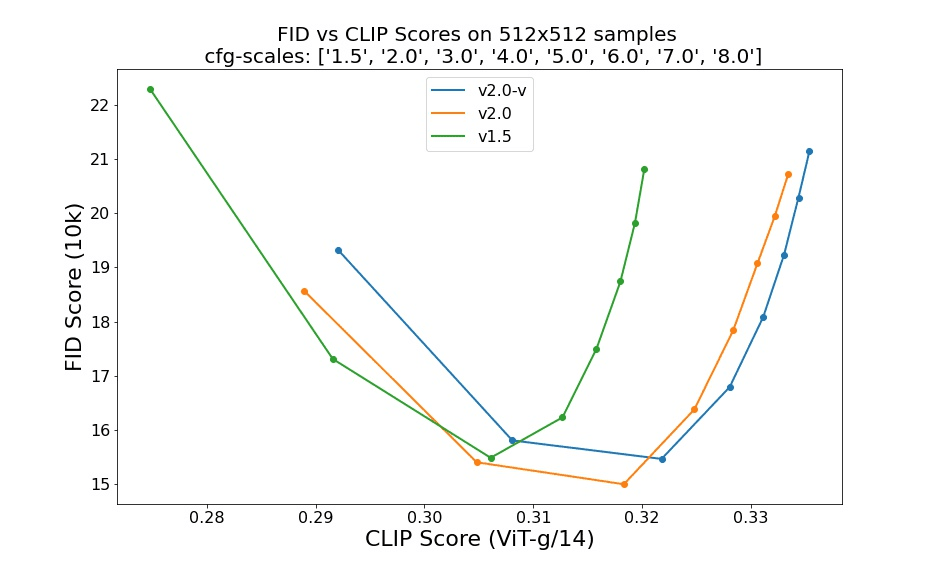
But is this the same for Dreambooth fine-tuning? Not necessarily. In fact, despite trying various approaches, we had problematic results using SD 2.0 and 2.1 in Dreambooth. In our experience, the process was nearly broken or at least extremely slow, relative to the 1.5 training.
While verifying our findings and searching the Internet we found mixed user feedback on Dreambooth + SD 2.0/1 and many similar observations that the 2.0 and 2.1 models are more difficult to fine-tune and it is much harder to generate art-style images with them.
We tried several things, including the use of different schedulers, and switching the encoder to OpenCLIP (used for training versions greater than 2.0). None of our attempts came close to the results from fine-tuning version 1.5. We are not saying that it is not possible, but you may wish to take this into account.
Note: the model weights we used in the comparison were pre-trained on 512×512 images to maintain the reliability of the comparison. It is not out of the question that SD 2.0 and 2.1 models pre-trained on higher-resolution images would have done better.
https://diffusion-charts.deepsense.ai/post03_chart005
Caption: Comparison of fine-tuning runs starting from different weights.
Inspecting the influence of prompt components and ‘magic words’
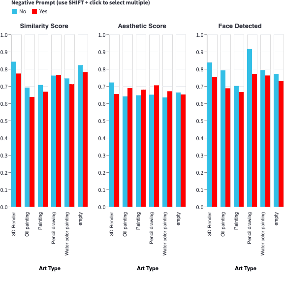
Thanks to our schematic approach to prompt engineering, we were also able to assess the individual parts of prompts in terms of the quality of pictures they produce. The results are presented after averaging 400,000 generations.
Different parts of the prompt have a specific impact on its quality; we hope that with this analysis you will be able to create better prompts!
https://diffusion-charts.deepsense.ai/post03_chart006
Caption: Comparison of key words from different categories used in the prompt, both with and without the use of a negative prompt.
Some of the useful insights regarding this analysis are:
- Significant differences can be seen in the presentation of the faces detected, which indicates that some parts of the prompts simply perform much better than others when it comes to the presentation of faces.
- Negative prompts improve aesthetics, but lower similarity levels and face-detection rates. The hypothesis explaining this phenomenon is that individual tokens lose their semantic meaning as the overall semantic load of the target image increases.
https://diffusion-charts.deepsense.ai/post03_chart007Caption: Overall average results of metrics for the use of negative prompts. Yes – when the negative was used, and No – when it was not.
Summary
In this blog post, we empirically investigated image generation using diffusion models. Imitating human evaluation, we objectively measured aspects usually left to subjective manual checks and arbitrary decisions. We carefully curated a diverse and representative dataset and a relevant prompt base (using a universal prompt template) to facilitate this investigation. Based on hours of experiments and proposed metrics, we investigated the data visually, gained a great deal of insight, and answered key questions concerning the quality of the generated images. You can use our findings in your facial image generations, and our approach can be used as inspiration and extended to other domains.
Appendix – Diversity calculation
Let’s denote as the set of generated images in a specific evaluation step by a specific model, represented by a set of n-dimensional embeddings.
The diversity measure considers each element of the set in relation to the other elements in the set. In other words, for each comparisons are made with each element of the set
. The following mean value is calculated for each element
:
Where is a cosine distance. The diversity score measure for the entire set
is obtained by calculating the mean value of the function
for the entire set
