R Notebook and Custom R Operations in the new Seahorse release

In this post, we present new features that come with Seahorse, Release 1.3 – the availability of writing custom operations, data exploration and ad-hoc analysis in R language using Jupyter Notebook. Along with Python (included in the previous Seahorse releases), R is one of the most popular languages in data science. Now, its users can embrace the new release of Seahorse with their favorite R operations included. Spark and R integration is obtained thanks to the SparkR package.

What’s new: R Notebook and custom R operations

There are several ways users can leverage R in their workflows. These include interactive Jupyter R Notebooks, custom R operations for processing data frames and tailor-made R evaluation functions. To demonstrate some of these new features, we are going to work with a dataset regarding credit card clients’ defaults available at the UCI Machine Learning Repository. We will train a model to predict the probability of a default of a loan. The dataset consists of 25 columns and 30K rows. Each row describes a customer of a bank along with information on his/her loan status. The last column – default_payment_next_month is our target variable. For a more detailed description of the dataset, please consult its description page and this paper.
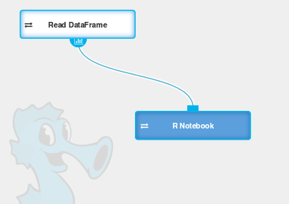
Having loaded the data, we proceed to its initial exploration. To this end, let’s use the R Notebook block from Seahorse’s operations palette.

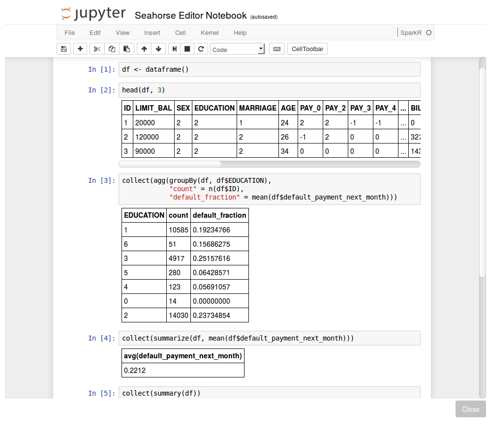
We open the Jupyter Notebook, and start exploring the data. With the use of the dataframe() function we are able to connect to data on the Spark cluster and operate on it. We can invoke it like this: df <- dataframe().

Some of the variables are categorical, for example: Education. In fact, reviewing the dataset documentation, we find that it is an ordinal variable where 0 and 6 denote the lowest and the highest education levels, respectively. In the notebook, after printing out the first three lines of data (the head() command), we performed a sample query for grouping the response variable with respect to education levels and compute the fraction of defaults within the groups. We observe some variability in default fraction with respect to education. Moreover, some of the categories are rare. In total, across all customers, the default fraction is equal about 22%.
Note the use of collect() functions here. This is a Spark-specific operation – it invokes the computation of an appropriate command and returns results to the driver node in a Spark application (in particular, it can be your desktop).
For later analysis we will drop the ID variable as it is irrelevant for prediction. We also see that there are relatively few occurrences of extreme values of the Education variable: 0 and 6 which denote the lowest and highest education levels, respectively. Our decision is to decrease the granularity of this variable and truncate its values to a range of [1, 5]. This can be achieved by a custom R Column Transformation as shown below.

Along with the Education variable, there are also other categorical variables in the dataset such as: marital status or payment statuses. We will not employ any special preprocessing for them since the model that we plan to use – Random Forest – is relatively insensitive to the encoding of categorical variables. Since most of the categories are ordinal, encoding them with consecutive integers is actually a natural choice here. For some other methods, like the logistic regression model, we would need to handle categorical data in a special way, for example, using one-hot-encoder.

To default or not to default

At this point we are ready to train a model. Let’s use the introduced Random Forest classifier, an off-the-shelf ensemble trees machine learning model. We devote 2/3 of data for tuning the model’s parameters – the number of trees in the forest and depth of a single tree – by Grid Search operation available on the palette. The other part of the data will be used for final model evaluation. Since the distribution of the target variable is slightly imbalanced toward “good” labels – about 78% customers in database paid their dues – we will use Area Under ROC as the evaluation metric. This metric is applicable when one class (label) dominates the other. It is more sensitive to retrieval of defaults in data rather than accuracy score (that is, the number of correctly classified instances regardless of their actual class).
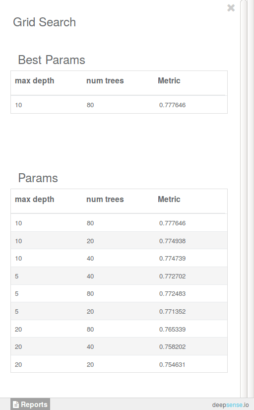
For demonstration purposes, we varied the parameters on a relatively small grid: 20, 40, 80 for the number of trees in the forest and 5, 10, 20 for tree depth. The results of the grid search are presented below:

We see that the optimal values for the number of trees and a tree depth are 80 and 10, respectively. Since there is little difference between choosing 20, 40 or 80 as the number of trees, we will stick with the smallest (and less complex) forest consisting of 20 trees as our final model.

Final check

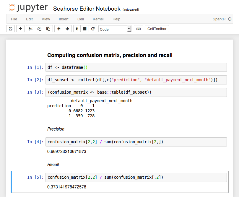
Finally, we evaluate the model on the remaining 1/3 part of data. It achieves a score of 0.7795 AUC on this hold-out dataset. This means that our model learned reasonably well to distinguish between defaulting and non-defaulting customers. For the sake of more interpretable results, the confusion matrix may be helpful. In order to compute it, we will create another R notebook and attach it to the final data with the computed predictions.

The confusion matrix is computed by retrieving two columns from the data frame and aggregating them. This, once again, is done using the collect() function. Here, it fetches the two selected columns to the driver node. Such operations should be performed with care – the result needs to fit into the driver node’s RAM. Here, we only retrieved two columns and there are merely 30K rows in the dataset so the operation succeeds. For larger datasets, we would order the computations to be performed by Spark. Finally, observe that we explicitly called the table() function from R’s base package via base::table(). This is necessary since the R native function is masked once SparkR is loaded.
Let’s proceed to the analysis of the confusion matrix. For example, its bottom left entry denotes that in 359 cases the model falsely predicted default while in fact there wasn’t one. Based on this matrix we may compute the precision and recall statistics. Precision is the fraction of correct predictions (true positives) out of all defaults predicted by our model. Recall is defined as the fraction of correctly predicted defaults divided by the total number of defaults in the data. In our application, precision and recall and equal about 67% and 37%, respectively.

The end

That’s it for today! We presented an analysis of prediction of defaults of a bank’s customers. Throughout the process, we used R for custom operations and exploratory data analysis. We trained the model, optimized and evaluated it. Based on costs associated with customers’ defaults, we can tweak precision and recall by, for example, adjusting the threshold level for probability of the default prediction and the final label (no default vs default) produced by the model. We encourage you to try out your own ideas – the complete workflow is available for download here.