Diagnosing diabetic retinopathy with deep learning

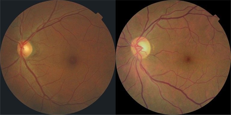
What is the difference between these two images?

The one on the left has no signs of diabetic retinopathy, while the other one has severe signs of it.

If you are not a trained clinician, the chances are, you will find it quite hard to correctly identify the signs of this disease. So, how well can a computer program do it?
In July, we took part in a Kaggle competition, where the goal was to classify the severity of diabetic retinopathy in the supplied images of retinas.
As we’ve learned from the organizers, this is a very important task. Diabetic retinopathy is the leading cause of blindness in the working-age population of the developed world. It is estimated to affect over 93 million people.
The contest started in February, and over 650 teams took part in it, fighting for the prize pool of $100,000.
The contestants were given over 35,000 images of retinas, each having a severity rating. There were 5 severity classes, and the distribution of classes was fairly imbalanced. Most of the images showed no signs of the disease. Only a few percent had the two most severe ratings.
The metric with which the predictions were rated was a quadratic weighted kappa, which we will describe later.
The contest lasted till the end of July. Our team scored 0.82854 in the private standing, which gave us 6th place. Not too bad, given our quite late entry.
You can see our progress on this plot:

Also, you can read more about the competition here.

Solution overview

What should be no surprise in an image recognition task, most of the top contestants used deep convolutional neural networks (CNNs), and so did we.
Our solution consisted of multiple steps:

• image preprocessing
• training multiple deep CNNs
• eye blending
• kappa score optimization

We briefly describe each of these steps below. Throughout the contest we used multiple methods for image preprocessing and trained many nets with different architectures. When ensembled together, the gain over the best preprocessing method and the best network architecture was little. We therefore limited ourselves to describing the single best model. If you are not familiar with convolutional networks, check out this great introduction by Andrej Karpathy: http://cs231n.github.io/convolutional-networks/.

Preprocessing

The input images, as provided by the organizers, were produced by very different equipment, had different sizes and very different colour spectrum. Most of them were also way too large to perform any non-trivial model fitting on them. A minimum preprocessing to make network training possible is to standardize the dimensions, but ideally one would want to normalize all other characteristics as well. Initially, we used the following simple preprocessing steps:

• Crop the image to the rectangular bounding box containing all pixels above a certain threshold
• Scale it to 256×256 while maintaining the aspect ratio and padding with black background (the raw images have black background as well, more or less)
• For each RGB component separately, remap the colour intensities so that the CDF (cumulative distribution function) looks as close to linear as possible (this is called “histogram normalization”)

All these steps can be achieved in a single call of ImageMagick’s command line tool. In time, we realized that some of the input images contain regions of rather intensive noise. When using the simple bounding-box cropping described above, this leads to very bad quality crops, i.e. the actual eye occupying an arbitrary and rather small part of the image.

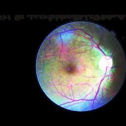
You can see gray noise at the top of the image. Using state of the art edge detectors, e.g. Canny, did not help much. Eventually, we developed a dedicated cropping procedure. This procedure chooses the threshold adaptively, exploiting two assumptions based on analysis of provided images:

• There always exists a threshold level separating noise from the outline of the eye
• The outline of the eye has an ellipsoidal shape, close to a circle, possibly truncated at the top and bottom. In particular it is a rather smooth curve, and one can use this smoothness to recognize the best values for the threshold

The resulting cropper produced almost ideal crops for all images, and is what we used for our final solutions. We also changed the target resolution to 512×512, as it seemed to significantly improve the performance of our neural networks compared to the smaller 256×256 resolution.
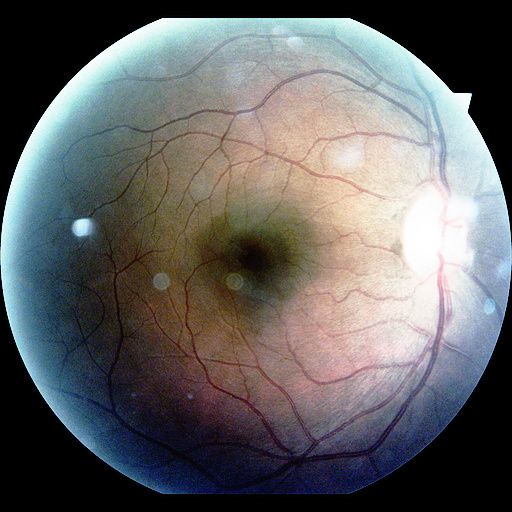
Here is how the preprocessed image looks like.

Just before passing the images to the next stage we transformed the images so the mean of each channel (R, G, B) over all images is approximately 0, and standard deviation approximately 1.

Convnet architecture

The core of our solution was a deep convolutional neural network. Although we started with fairly shallow models — 4 convolutional layers, we quickly discovered that adding more layers, and filters inside layers helps a lot. Our best single model consisted of 9 convolutional layers.
The detailed architecture is:

| Type    | nof filters | nof units |
|---------|-------------|-----------|
| Conv    | 16          |           |
| Conv    | 16          |           |
| Pool    |             |           |
| Conv    | 32          |           |
| Conv    | 32          |           |
| Pool    |             |           |
| Conv    | 64          |           |
| Conv    | 64          |           |
| Pool    |             |           |
| Conv    | 96          |           |
| Pool    |             |           |
| Conv    | 96          |           |
| Pool    |             |           |
| Conv    | 128         |           |
| Pool    |             |           |
| Dropout |             |           |
| FC1     |             | 96        |
| FC2     |             | 5         |
| Sofmax  |             |           |

All Conv layers have 3×3 kernel, stride 1 and padding 1. That way the size (height, width) of the output of the convolution is the same as the size of the input. In all our convolutional layers we follow the convolutional layer by batch normalization layer and ReLu activations. Batch normalization is a simple but powerful method to normalize the pre-activation values in the neural net, so that their distribution does not change too much during the training. One often standardizes the data to make zero mean and unit variance. Batch normalization takes it a step further. Check this paper by Google to learn more. Our Pool layers always use max pooling. The size of the pooling window is 3×3, and the stride is 2. That way the height and width of the image get halved by each pooling layer. In the FC (fully connected) layers we again use ReLu as activation function. The first fully connected layer, FC1 also employs batch normalization. For regularization we used Dropout layer before the first fully connected layer, and L2 regularization applied to some of the parameters.
Overall, the net has 925,013 parameters.
We trained the net using stochastic gradient descent with momentum and multiclass logloss as a loss function. Moreover, the learning rate has been adjusted manually a few times during the training. We have used our own implementation based on Theano and Nvidia cuDNN.
To further regularize the network, we augmented the data during the training by taking random 448×448 crops of images and flipping them horizontally and vertically, independently with probability 0.5. During the test time, we took few such random crops, flips for each eye and averaged our predictions over them. Predictions were also averaged over multiple epochs.
It took quite long to train and compute test predictions even for a single network. On a g2.2xlarge AWS instance (using Nvidia GRID K520) it took around 48 hours.

Eye blending

At some point we realized that the correlation between the scores of two eyes in a pair was quite high. For example, the percent of eye pairs for which the score for the left eye is the same as for the right one is 87.2%. For 95.7% of pairs the scores differ by at most 1, and for 99.8% by at most 2. There are two likely reasons for this kind of correlation.
The first is that the retinas of both eyes were exposed to the damaging effects of diabetes for the same amount of time, and are similar in structure, so the conjecture is that they should develop the retinopathy at similar rate. The less obvious reason is that the ground truth labels were produced by humans, and it is conceivable that a human expert is more likely to give the same image different scores, depending on the score of the other image of the pair.
Interestingly, one can exploit this correlation between the scores of a pair of eyes to produce a better predictor.
One simple way is to take the predicted distributions D_L and D_R for the left and right eye respectively and produce new distributions using linear blending, as follows. For the left eye, we predict c⋅D_L+(1-c)⋅D_R, similarly we predict c⋅D_R+(1-c)⋅D_L for the right eye, for some c in [0, 1]. We tried c = 0.7 and a few other values. Even this simple blending produced a significant increase in our kappa score. However, a much bigger improvement was gained when instead of an ad-hoc linear blend we trained a neural network. This network takes two distributions (i.e. 10 numbers) as inputs, and returns the new “blended” versions of the first 5 inputs. It can be trained using predictions on validation sets. As for the architecture, we decided to go with a very strongly regularized (by dropout) one with two inner layers of 500 rectified linear nodes each.
One obvious idea is to integrate the convolutional networks and the blending network into a single network. Intuitively, this could lead to stronger results, but such a network might also be significantly harder to train. Unfortunately, we did not manage to try this idea before the contest deadline.

Kappa optimization

Quadratic weighted kappa (QWK), the loss function proposed by the organizers, seems to be a standard one in the area of retinopathy diagnosis, but from the point of view of mainstream machine learning it is very unusual. The score of a submission is defined to be one minus the ratio between the total square error of the submission (TSE) and the expected squared error (ESE) of an estimator that answers randomly with the same distribution as the submission (look here for a more detailed description).
This is a rather hard loss function to directly optimize. Therefore, instead of trying to do that, we use a two-step procedure. We first optimize our models for multiclass logloss. This gives a probability distribution for each image. We then choose a label for each image by using a simulated annealing based optimizer. Of course we cannot really optimize QWK without knowing the actual labels. Instead, we define and optimize a proxy for QWK, in the following way. Recall that QWK = 1 – TSE/ESE. We estimate both TSE and ESE by assuming that the true labels are drawn from the distribution described by our prediction, and then plug these predictions into the QWK formula, instead of the true values. Note that both TSE and ESE are underestimated by the procedure above. These two effects cancel each other out to some extent, still our predictions QWK were off by quite a lot compared to the leaderboard scores.
That said, we found no better way of producing submissions. In particular, the optimizer described above outperforms all the ad-hoc methods we tried, such as: integer-rounded expectation, mode, etc.

We would like to thank California Healthcare Foundation for being a sponsor, EyePACS for providing the images, and Kaggle for setting up this competition. We learned a lot and were happy to take part in the development of tools that can potentially help diagnose diabetic retinopathy. We are looking forward to solving the next challenge.

deepsense.ai Machine Learning Team