Diffusion models in practice. Part 1: A primers
The AI revolution continues, and there is no indication of it nearing the finish line. The last year has brought astonishing developments in two critical areas of generative modeling: large language models and diffusion models. To learn more about the former, check out other posts [1] by deepsense.ai. This series is devoted to sharing our practical know-how of diffusion models.
Application of the family of models using a mechanism called “diffusion” in various generative setups remains one of the hottest topics in machine learning. Diffusion-based models have proven their ability to yield results surpassing all other well-known counterparts used in this domain beforehand, such as Generative Adversarial Networks (GANs) or Variational Autoencoders (VAEs). Sohl-Dickstein et al.’s [2] publication in 2015 brought a breath of fresh air to the generative model scene. For a few years, the concept was gradually improved upon, and just last year there were numerous state-of-the-art publications in the domain of image-to-image, text-to-audio, and time series forecasting, just to name a few. The number of applications is growing by the day, although the text-to-image domain remains the most popular so far – we are focusing solely on it in this series as well. There are many practical questions one may have when trying to use these methods, such as:
- Which tools bring the best results?
- How can I reliably judge whether the results are satisfactory?
- What parameter values should I use in image generation?
- How many images should I use to train diffusion models optimally? How many training steps?
These and similar questions have both beginners and advanced practitioners struggling. While the Internet is full of math-heavy theories and opinionated claims, there are not many well-researched answers to these questions available. Over the next few posts, we intend to present a practical and empirical answer to them.
The series will contain the results of multiple experiments using various models and metrics. Based on these, we will present insights which are relevant to the specific practical dilemmas and challenges, and allow you to draw your own conclusions by facilitating a graphical, interactive exploration of these results.
First, however, this post will lay the groundwork for this with just enough theory to make the following ones understandable. We will introduce the relevant tools and concepts to be referenced in later posts, and we strongly recommend familiarizing yourself with them. More specifically, we will introduce Stable Diffusion [3] (one of the loudest models published last year) and several tools used to finetune it, including DreamBooth [4], LoRA [5], and Textual Inversion [6].
Stable Diffusion: the root of it all
While DALL·E [7] and DALL·E 2 [8] were responsible for drawing large-scale attention to generative image models, Stable Diffusion [3] was the model that unleashed a true revolution. Since its open-sourcing in August 2022, anyone could modify, expand, tweak, or simply use it on their GPU or in a collab [9] for free. Follow-up technologies appeared, including training methods like DreamBooth [4], allowing people to see themselves (or anyone else) as a character in their generative art. The landscape of generative models (and possibly of art itself [10]) changed forever.
What does ‘diffusion’ stand for in ‘diffusion models’ and ‘Stable Diffusion’?
While ‘Stable Diffusion’ sounds catchy, for someone starting their adventure in the generative realm, the term ‘diffusion’ may be confusing. Within the context of deep learning, diffusion refers to one of the processes used by these methods to generate images based on the training data. That is, admittedly, a bit vague. How exactly do diffusion models differ from GANs, VAEs, or other models used in image modeling?
There are numerous novelties proposed. Essentially, various generative architectures are composed of two processes that are complementary to each other. GANs architectures utilize a generator and discriminator, while VAEs use an encoder and decoder setup. For diffusion-based models, it is no different, as we can formulate the model with two processes – diffusion (noising) and denoising [11].
Diffusion – also referred to as the forward diffusion process – is meant to sequentially destroy the image by slowly blurring the picture so that its main characteristics are no longer observable. One of the relatively new ideas for this family of models is that the formulation of this forward process is fixed. That is a large difference when compared to, e.g., VAEs, where both main components of the architecture are fully trainable. In the case of diffusion, the encoder’s job is overtaken by a mathematical process – the neural network approach is redundant.
The main goal of the entire architecture is to teach the model to reverse that process; to create something meaningful – an image – from a complete noise. This denoising process is performed by a neural network, and arguably this is the place where most of the heavy lifting is done. During the training, the network is presented with a diffused image and is taught to predict the noise added to it. When the predicted noise is subtracted from the input, a person/object/scene starts to emerge in the picture. As usual, the network is trained on millions of images and the feedback about its performance is constantly provided via loss function and backpropagation. The whole process allows the network to gather information about the characteristics of the pictures from the same class. We don’t tell the network explicitly how to reverse the diffusion process, since the generative power comes from the interpolation of the knowledge that the model gains during the training. Truth is, we wouldn’t even be able to do that, since it would require the model to have virtually infinite capacity (more about this in detail in [12]).
That’s a very brief summary of the basics of the construction of diffusion models. We already have a detailed blog post [12] that focuses on the mathematical aspects. We covered DALL·E 2 [8] and Imagen [13] in detail there – we strongly recommend checking it out, as it should shed a great deal of light on the intricacies of diffusion in deep learning. In this section, we will give a general overview of the key terms and components of Stable Diffusion.
The building blocks
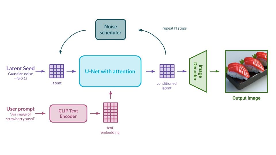
Even though the image above might indicate otherwise, compared to the intricate architecture of e.g. DALL·E 2 [8], Stable Diffusion [3] seems to be based on concepts which are a little easier to grasp. There are three main components of the solution:- Text Encoder, which is necessary for translation between the text and the latent generative space,
- U-Net type Neural Network, which runs the diffusion process allowing for the generation of new information,
- Image Autoencoder, which is able to compress the input image into its latent space representation and translate the latent output into the actual image.
Below we will explain each of these in a bit more detail.
Text Encoder
Diffusion models can work on their own, generating images based on the knowledge gained through the training process. Usually, we would like to be able to guide the generation process using text, so the model produces exactly what we want. This information is passed into the model in the form of a generation prompt. So how does the model understand the text?
When it comes to text-to-image generation, we can have the best of the generative and natural language processing worlds and successfully apply the solutions from one domain to the other. The area of Language Models has gained momentum rapidly in recent years. An increasing number of solutions allow for efficient embedding of the text in the abstract space, which later allows for efficient processing of the text in hand.
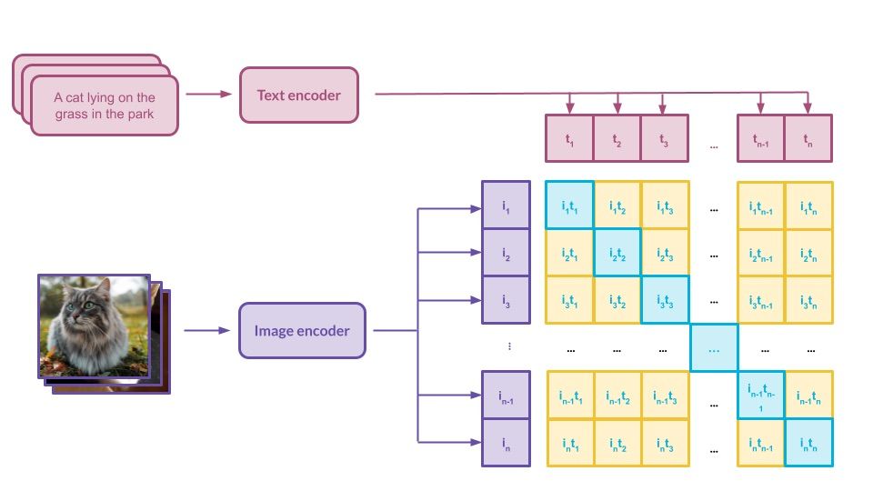
The idea of a text encoder is quite simple – we wish to take the textual input and represent it efficiently in a space that would allow the model to generate an image based on the prompt. That process is called text guidance – each time the diffusion model goes one step further in the image generation process, it is reminded of what the image was supposed to present. Currently, the choice of the model that transfers the text into a latent space seems paramount for accurate and high-quality generation. Many of the current state-of-the-art solutions utilize different architectures for text embedding. For instance, Imagen [13] architecture uses the T5-XXL [14], while Stable Diffusion uses the CLIP ViT-L/14 model [15] to get the job done.
CLIP [16] was trained with millions of (text, image) pairs and can accurately map the text to the image and vice versa. This makes it a very natural choice for the embedder, and it has already been proven to perform well, e.g., in DALL·E. The model itself is pre-trained and fixed in the Stable Diffusion, although there are ways to interfere with the embeddings – we will talk about those later in this post.
U-Net type Neural Network
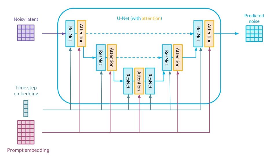
The heart of the solution – this part of the architecture takes the embedded text and noised latent and tries to reverse the diffusion process in a way that would produce an image as similar to the input prompt as possible. For anyone that follows neural network evolution, the way this is done may not be a great surprise. The weapon of choice is U-Net architecture, which was already used for lots of diffusion architectures before Stable Diffusion.
The denoising process happens step-by-step – each ResNet block receives the information about the denoising step and the text embedding is processed by the attention mechanism. A neural network aims to predict the noise that was added to the image during a forward pass of diffusion – that’s why the information about the step is important. During inference, the network tries to produce an image from a randomly sampled latent. The authors opted for the already well-established solution incorporating classifier-free guidance [17] to make sure that the image output is as close to the input text as possible.
Image Autoencoder
The diffusion process itself is not very lightweight. Multiplying the height and width of the image, the number of color channels, and the number of noising steps in the process already leads to numerically heavy calculations. The authors of Stable Diffusion decided to address that by transferring the main part of the diffusion process into the latent space. Essentially the idea is to perform denoising not on the actual image in pixel dimensions, but rather to do it on a latent representation of the image, which is compressed to yield fewer dimensions. Historically there were already a few ways of performing this type of compression – the authors opted for an already well-known autoencoder approach.
During the training, the input image is processed by the encoder and represented as latent several times smaller than the original e.g. 3x512x512 image is represented as a 6x64x64 matrix. It means that, in the architecture, all models work with a compressed representation of inputs that retains only the most valuable information. After the reverse diffusion process happens in U-Net, the tensor with all the necessary information for image generation is translated into the actual picture by the decoder.
To sum up, the flow seems easy enough – we type the text, and the encoder translates the text into a concise embedded form. The main model reverses the diffusion process of random noise in a step-by-step fashion, at the same time conditionally guiding the generation using the text. The last step is to take the model output and generate an image – that is the image decoder’s job. Our goal was to explain the interior of this architecture as simply as possible, but it needs to be underlined that actual model usage and navigating through the different parameters and settings is far more difficult! Worry not, as we will be helping with that as well.
Newer is better? v2.x vs v1.x
November 2022 brought another iteration of the Stable Diffusion architecture – Stable Diffusion 2.0 [18]. Two weeks later, in December, Stability AI published the most recent stable version of the flag model to date – version 2.1 [19]. Just like its predecessor, it is available in the form of a demo [20]. There were a couple of major tweaks compared to the 1.5 version.
The new text encoder and dataset choice seem to be the largest of the changes. This time a newer generation OpenCLIP-ViT/H [21] model was trained to handle the task of text embedding. Just like its predecessor, CLIP ViT-L/14, its weights are open-sourced. The dataset used for the OpenCLIP training is open and includes several changes that drastically altered the way that model works with the prompts. An additional NSFW filter was included to filter out the images that could lead to misuse across the internet, mostly related to child abuse and pornography. Also, there is a noticeably smaller collection of celebrities and artistic images.
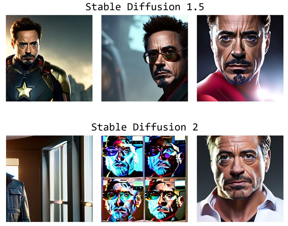
Comparison of generation for the prompt: “a studio photograph of Robert Downey Jr., cinematic lighting, hyperdetailed, 8 k realistic, global illumination, radiant light, frostbite 3 engine, cryengine, trending on artstation, digital art” for SDv1.5 and SDv2.0. Source: [22]
Additionally, negative prompting seems to be more important for accurate generation in the newer versions of Stable Diffusion. Negative prompts are appended to the regular generation prompt and should retain the information of what should not be seen on the generated picture. It was highly optional for the first version of the architecture, but it seems to be a must in the 2.0 and 2.1 versions in order to get high-quality results.
![Example of the importance of negative prompting in the 2.1 version. The pictures on both the left and right were generated with the same prompt, but there was an additional negative prompt added on the right to reduce the greenery in the image. Source: [19]](https://deepsense.ai/wp-content/uploads/2023/03/Example-of-the-importance-of-negative-prompting-in-the-2.1-version.jpeg.pagespeed.ce.zCpaNzfP9T.jpg)
Example of the importance of negative prompting in the 2.1 version. The pictures on both the left and right were generated with the same prompt, but there was an additional negative prompt added on the right to reduce the greenery in the image. Source: [19]
Training tools
Although generative models offer endless possibilities, their domain knowledge can be limited. Often, the generation process relies on interpolating between images seen during training. While general pre-trained models are versatile, specific use cases may require additional training of the model. Since the release of Stable Diffusion as open-source software, several techniques have emerged to extend the knowledge of pre-trained models, collectively known as fine-tuning.
Several methods have been developed to generate specific objects, styles, or compositions with minimal data requirements. These techniques have pushed the boundaries of generative art even further. In the following chapters, we describe some established fine-tuning methods, some of which we used in our experiments.
DreamBooth
This is one of the most popular methods, designed mainly to extend the model’s knowledge to include specific objects, but it is also possible to introduce styles (e.g. to incorporate a new artist). It works great for placing the face of a particular person in the model’s domain and more. It was also this method that we used for our internal Christmas card generator project – feel free to check it out [23].
When it comes to the technicalities, DreamBooth [4] is quite close to the traditional definition of fine-tuning.
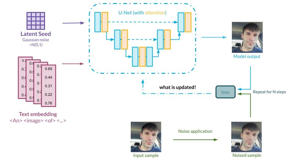
In its basic form, it relies on freezing all weights of the architecture except for the U-Net model, which runs the denoising process. Additional training of the model is based on iteratively showing the network sample images of, e.g., the object of interest, along with a prompt containing a new, unique identifier to symbolize it, e.g., “A photo of a <identifier> dog”. The idea is to embed the knowledge about an object within the model weights and force it into the embedding layer. In the publication [4] the authors present a method for the rare-token selection to link with the identifier. The importance of choosing sparse tokens in this operation is not to be neglected – the model might lose some important information in the process.
Additionally, to combat overfitting and language drift, some regularization images with similar prompts are also shown during fine-tuning to ensure that the network does not forget the original meaning of the remaining tokens – this idea is called prior-preservation loss.
It is worth mentioning that DreamBooth implementation provided by Hugging Face [24] allows you to unfreeze the weight of the text encoder as well, which can further improve the results. On the other hand, it requires so much computing power that only a small percentage of users can launch these tools on their local machines. DreamBooth itself reigns supreme in terms of popularity among all methods listed in this post, but it comes with a price – it is the most computationally expensive. Even with the most basic setup, including numerous memory-efficient optimizations, this way of fine-tuning needs a GPU with 12GB of VRAM to perform training without major complications.
As of today, there are already hundreds of different concepts in the concepts library setup on Hugging Face – we strongly recommend checking them out [25].
LoRA
LoRA [5] stands for Low-Rank Adaptation. It is not a diffusion-specific concept, as it was published in 2021 and targeted the problem of fine-tuning large language models such as GPT-3 [26]. These models, with millions of parameters, require a lot of storage, and altering the whole architecture each time there can be computationally expensive. Generally speaking, models are defined by parameters, which are stored in matrices. As the dimensions of the model increase, these matrices can grow very rapidly, which makes them heavy.
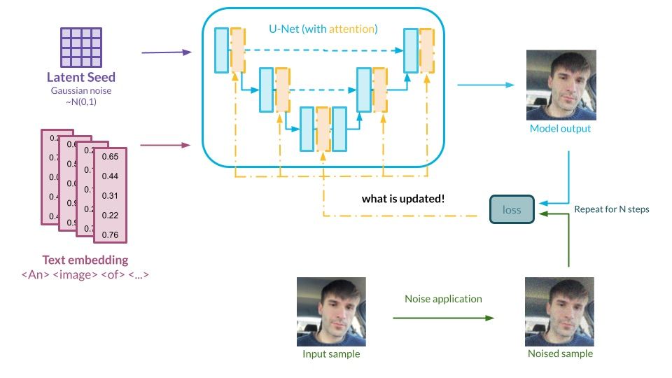
In a nutshell, LoRA is a technique used to reduce the number of parameters that need to be tweaked to fine-tune the model. Instead of working with the whole matrices of parameters, these matrices are converted into a lower rank decomposition, which makes their size magnitudes smaller. On top of that, this technique does not need to be applied everywhere in the model. In the context of diffusion architectures – such as Stable Diffusion – the attention layers in the UNet network are specifically targeted, as they directly link the textual semantics with the generative ability of the model.
This approach yields several advantages:
- Most of the pre-trained weights are frozen and unaffected by this operation, which should ensure that the generative power of the model remains the same after fine-tuning,
- Sharing the tweaked model is much easier as the changes boil down to a lightweight diff-like file,
- Fewer parameters to train = faster results; this method also works with just a couple of images required.
Textual Inversion
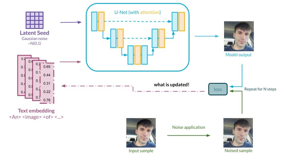
Another powerful yet simple technique that can be used for adding new concepts to the model is called textual inversion [6]. It works by directly interfering with the text embedding layer of the architecture. The idea is similar to that of DreamBooth – we wish to give the model some information about a certain concept, potentially a new object or style, while maintaining the existing information.
This procedure boils down to adding a new token to the vocabulary, for instance <custom_woman_token>, and initializing its embedding to be the same as for the already existing <woman> token. Next, by providing a set of images corresponding to that new token, the idea is to fine-tune the embedding rather than the model, which remains frozen. We want to find optimal embedding so that the characteristics of the object are well captured. The advantage of such an approach is that the results are lightweight and easy to share – embedding tensors have only a few kilobytes.Hugging face offers a space [27] that showcases different new concepts that have been introduced into the embedding space of Stable Diffusion, such as <midjourney-style> or <nebula>.
A lot of room for exploration
The use of different training techniques and ways to customize models is an area which is developing much faster than the traditional architecture research related to diffusion models. Here we have covered just the three most popular ways to fine-tune the model, but developers are constantly testing new ways to interact with the model, such as Hypernetworks training [28]. On top of that, there are ways to combine several methods for an even more powerful effect. For instance, one could combine Textual Inversion with LoRA, first by tuning the new embedding and then tuning the diffusion mechanism using images related to the newly embedded object.
From the practical perspective, there is no one-size-fits-it-all method; as usual, each comes with a certain trade-off. DreamBooth seems to be yielding great results, but it is computationally and spatially expensive. Textual Inversion is highly lightweight but it is limited to the model’s idea of embeddings. LoRA sits in the middle, combining a bit of both – not as lightweight, but it does interact with the model’s weights directly.
Summary
In this article, our goal was to arm the reader with the knowledge necessary to understand where the diffusion models are right now in the context of text-to-image generation. We also wanted to share the overview of popular methods related to the training itself, as it is a vital part of today’s development.
“But which method should be used? And how?” – these are the questions that we want to address in the next posts from this series. We will be looking a lot closer at the practical side of things – there will be training, optimization, validation, and more – stay tuned!
References
- https://deepsense.ai/blog/
- Deep Unsupervised Learning using Nonequilibrium Thermodynamics, Sohl-Dickstein et al. 2015
- High-Resolution Image Synthesis with Latent Diffusion Models, Rombach et al. 2022
- DreamBooth: Fine Tuning Text-to-Image Diffusion Models for Subject-Driven Generation, Ruiz et al. 2022
- LoRA: Low-Rank Adaptation Of Large Language Models, Hu et. al. 2021
- An Image is Worth One Word: Personalizing Text-to-Image Generation using Textual Inversion, Gal et al. 2022
- Zero-Shot Text-to-Image Generation, Ramesh et al. 2021
- Hierarchical Text-Conditional Image Generation with CLIP Latents, Ramesh et al. 2022
- https://colab.research.google.com/github/huggingface/notebooks/blob/main/diffusers/stable_diffusion.ipynb
- https://hbr.org/2022/11/how-generative-ai-is-changing-creative-work
- Denoising Diffusion Probabilistic Models, Ho et al. 2020
- The recent rise of diffusion-based models, deepsense.ai, 2022
- Photorealistic Text-to-Image Diffusion Models with Deep Language Understanding, Saharia et al. 2022
- How Much Knowledge Can You Pack Into the Parameters of a Language Model?, Roberts et al. 2020
- https://huggingface.co/sentence-transformers/clip-ViT-L-14
- Learning Transferable Visual Models From Natural Language Supervision, Radford et al. 2021
- Classifier-Free Diffusion Guidance, Ho et al. 2021
- https://stability.ai/blog/stable-diffusion-v2-release
- https://stability.ai/blog/stablediffusion2-1-release7-dec-2022
- https://huggingface.co/spaces/stabilityai/stable-diffusion
- https://github.com/mlfoundations/open_clip
- https://www.assemblyai.com/blog/stable-diffusion-1-vs-2-what-you-need-to-know/
- https://deepsense.ai/portfolio-item/christmas-card-generator
- https://github.com/huggingface/diffusers/tree/main/examples/dreambooth
- https://huggingface.co/sd-dreambooth-library
- Language Models are Few-Shot Learners, Brown et al. 2020
- https://huggingface.co/spaces/sd-concepts-library/stable-diffusion-conceptualizer
- HyperNetworks, Ha et al. 2016


![Stable Diffusion architecture, source: [3]](https://deepsense.ai/wp-content/uploads/2023/03/Stable-Diffusion-architecture.jpeg.pagespeed.ce.fYgD_oefV5.jpg)
![Inverting a visual idea of a specific cat into a <S∗> token. Source: [6]](https://deepsense.ai/wp-content/uploads/2023/03/Inverting-a-visual-idea-of-a-specific-cat-into-a-token.jpeg)
