Evaluations, Limitations, and the Future of Web Agents – WebGPT, WebVoyager, Agent-E
Web Agents are no longer just a concept from science fiction—they’re the cutting-edge tools that are automating and streamlining our online interactions at an unprecedented scale. From effortlessly sifting through vast amounts of information to performing complex tasks like form submissions and website navigation, these agents are redefining efficiency in the digital age.
Thanks to groundbreaking advancements in Large Language Models (LLMs), we’re witnessing a paradigm shift. The humble beginnings of web scraping and archiving have rapidly evolved. Now, sophisticated agents like WebGPT and WebVoyager don’t just perform tasks; they understand context, interpret nuances, and mimic human browsing behavior in ways we once only imagined. They’re not just faster—they’re smarter.
But with great power comes great complexity. The real world isn’t a controlled environment, and web agents face formidable challenges. Dynamic content, ever-changing web landscapes, intricate user interactions—the hurdles are significant. Current systems, while advanced, are just scratching the surface of what’s possible.
This article isn’t just an overview; it’s a journey into the heart of web agent technology. We’ll explore the state-of-the-art solutions making waves today, delve into the intricacies of evaluating their performance, and spotlight the key obstacles that innovators are racing to overcome.
Whether you’re a business leader looking to harness this technology for a competitive edge or a tech professional eager to dive into the next big thing, understanding web agents is crucial. The future of web interaction is here, and it’s more exciting—and challenging—than ever before.
TL;DR – Web Agents: From Browsing to Automation
Forget bots that just scrape data—Web Agents are like having little AI assistants navigating the web for you. Need info buried deep in a website? Want to automate a tedious online task? These AI-powered tools are stepping up their game, using LLMs to understand and interact with websites like never before.
Key takeaways:
- Forget basic bots—Web Agents are leveling up. They’re starting to understand context, interpret nuances, and browse the web in a way that’s more like us humans.
- WebGPT, an early pioneer, uses text-based browsing to answer questions more accurately than traditional LLMs.
- WebVoyager, powered by GPT-4v, utilizes visual input and the “Set-of-Mark” method to navigate real websites, overcoming challenges like dynamic content.
- Agent-E introduces advanced HTML distillation techniques and a multi-agent architecture for efficient task execution and resource utilization.
- Evaluating Web Agents requires new benchmarks: WebArena and WebVoyager’s evaluation framework offer realistic scenarios and diverse tasks to assess agent performance.
- Limitations still exist: Handling complex web actions, file compatibility, integrating multimodal inputs, and ensuring ethical and secure deployment are ongoing challenges.
- The future is promising: Combining textual and visual inputs, improving robustness, and developing standardized evaluation methods will pave the way for wider adoption.
The Fundamentals of Web Agents
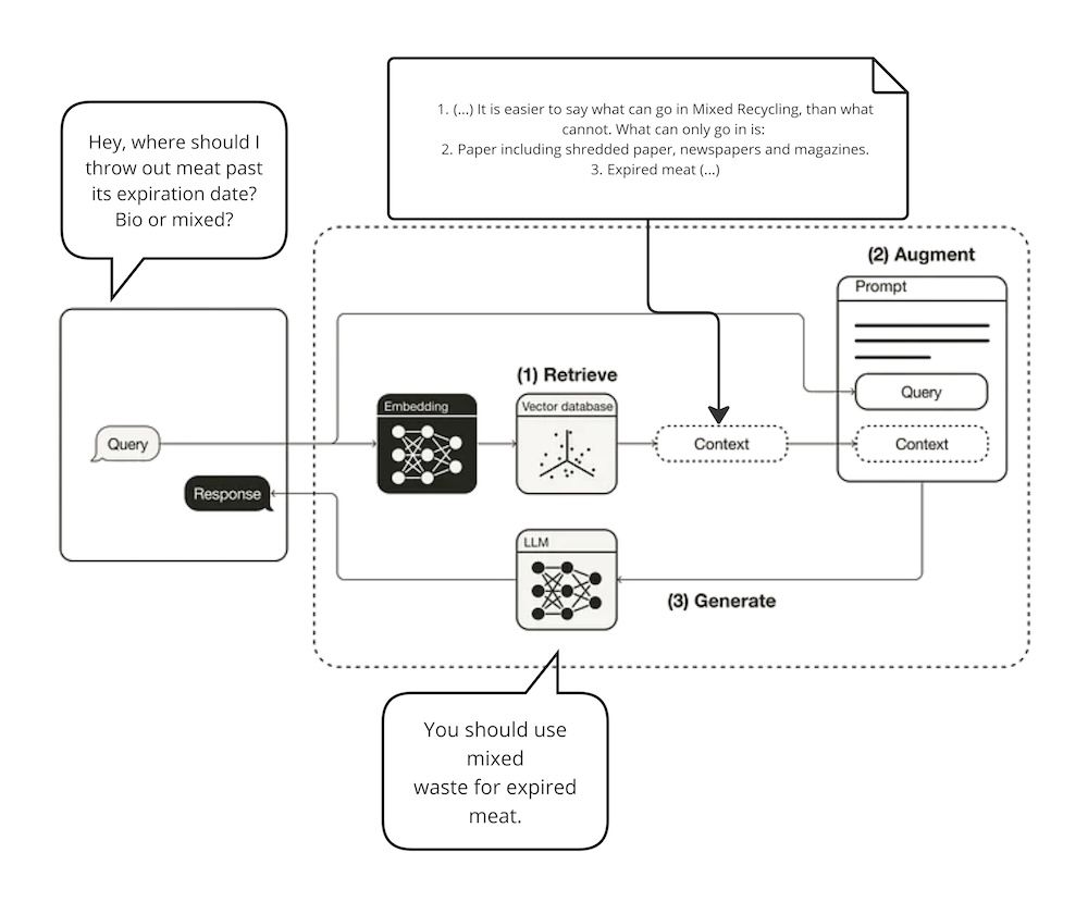
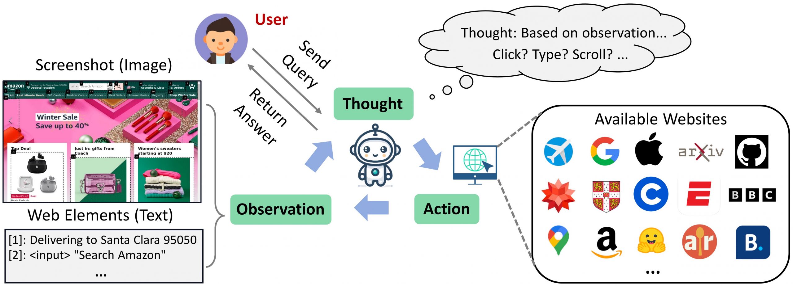
The basics of Web Agents aren’t that different from regular AI Agents used in other fields. A pretty matching, though obviously very simplistic definition of an LLM-based AI Agent is that it is an LLM put into a loop. The diagram below shows how Web Agents work.
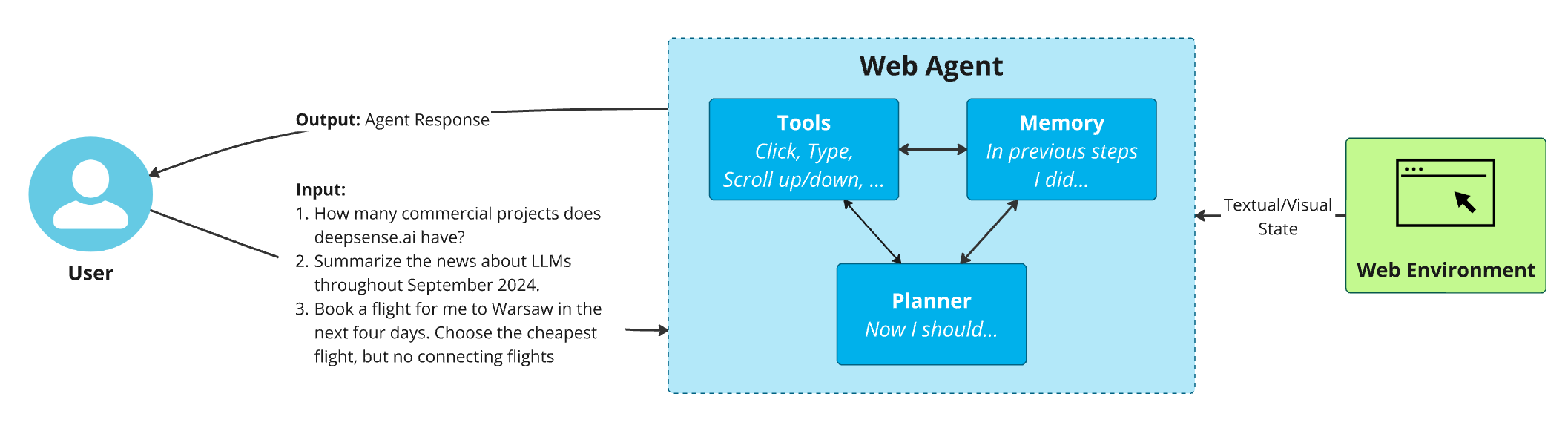
Components of Web Agent, source: own study
Here are the main parts of such a system:
- Planning: Based on the user’s request, the agent makes a plan.
- It might get a detailed step-by-step guide and schedule all tasks at the beginning for future execution.
For example, if the Web Agent is to operate on a concurrent web service with good documentation explaining the process to follow (e.g. in Sharepoint or Confluence), specific fields to fill in and buttons to click, the Web Agent can decompose this as a ready-made action plan. - Alternatively, the agent might only receive the expected outcome from the user and be required to formulate a step-by-step plan in real-time. The agent, based on feedback from the web environment, has to plan the next step.
For example, “My task is to edit the user’s profile. I see an icon with the user’s avatar, so I’m guessing I can click on it to go to the profile”.
- It might get a detailed step-by-step guide and schedule all tasks at the beginning for future execution.
- Tools: Following the plan, the agent carries out actions.
- It could be some predefined actions like “click”, “type”, “scroll up/down” or “go back”.
- Another option – our agent might have the freedom to write code on the fly using tools like Selenium or Playwright.
- Memory: The agent needs to remember what it did previously. This allows it to review past steps and figure out what to do next and how to do it.
For example, “My task is to edit the user’s profile. I see an icon with the user’s avatar, but I tried clicking on it before and nothing happened. Therefore, I will try…”
An additional component is the feedback from the Web Environment. At each step, it’s crucial to gather information from the browser regarding the current on-screen content. This data can include HTML code or, thanks to recent advances in vision language models, screenshots of the page, which align the web agent’s perspective more closely with that of the human user.
Such systems can be enhanced in various directions. Here are some examples of user queries to illustrate their versatility:
- “How many commercial projects does deepsense.ai have?”: A straightforward query focusing primarily on extracting information from a single source.
- “Summarize the news about LLMs throughout September 2024.”: This scenario may require intelligent aggregation of source data and subsequent processing.
- “Book a flight for me to Warsaw in the next four days. Choose the cheapest flight with no connecting flights.”: Here, in addition to passively browsing through websites, we perform specific actions with permanent outcomes. (Quite a responsible task for a dummy AI agent, huh?)
Web Agents can be tailored for a variety of tasks, proving to be incredibly flexible and useful in different scenarios.
Overview of Web Agent Solutions: Differences Between WebGPT, WebVoyager and Agent-E
WebGPT: the first LLM-based web agent
Looking back, we can remember web archiving and web scraping tools – technologies that have been on the market for years and can be considered early forms of Web Agents. However, the introduction of LLMs allowed for far more intricate and less monotonous processes. Efforts to achieve this complexity predated even the first release of ChatGPT! Staying within OpenAI’s innovative endeavors, 2021 saw the launch of WebGPT.
Back then, it was already acknowledged that models tend to “hallucinate” or provide inaccurate information. To address this, WebGPT uses search queries, follows links, navigates pages, and looks for pertinent answers, emulating human browsing behavior within a text-based web browser created by its developers.
The model kicks off with an open-ended question and a summary of the browser state, then issues commands like “Search …”, “Find in page: …” or “Quote: …” to gather and compile information into an answer.
Showcase of WebGPT, source: https://openai.com/index/webgpt/
While WebGPT is more accurate than GPT-3 (the model on which it is based), it still commits basic errors and can perpetuate users’ biases. The citations it generates can lend an undue sense of credibility, potentially disguising the inherent inaccuracies and errors.
WebVoyager: Utilizing Vision Language Models for Browsing the Web
Although early attempts at developing LLM-based web agents began as far back as 2021 with WebGPT, it wasn’t until the summer of 2024 that two significant research papers emerged, each examining the topic from distinct perspectives. The first noteworthy work is WebVoyager, an agent that makes decisions based on its visual input, leveraging the multimodal capabilities of GPT-4v.
Workflow overview
When given an instruction, WebVoyager launches a web browser and takes actions guided by screenshots from the web. At every step, the agent evaluates the screenshot with possible options marked and decides on the next action, which is then executed in the browser environment. This sequence of actions continues until the agent determines that the task is complete and decides to stop.
Workflow of WebVoyager, source: https://arxiv.org/pdf/2401.13919
The authors of WebVoyager created an automated web-browsing environment utilizing Selenium. In contrast to WebGPT, which functions within an artificial setting, WebVoyager allows the agent to navigate the open web, encountering distinct challenges like floating ads, pop-up windows, and continuous updates. They chose real-time interaction with live websites to more accurately mirror real-world scenarios, where agents need to access up-to-date information from the web.
Set-of-mark. How the AI-powered wWeb Agents Perceive the World
Much like how humans explore the web, WebVoyager uses visual data, specifically screenshots, as its primary input. This approach avoids the complexity of parsing the HTML DOM tree or accessibility tree, which can often generate excessively verbose text and complicate the language model’s decision-making process. WebVoyager utilizes the innovative Set-of-Mark method to overlay bounding boxes over interactive elements on websites, guiding the agent’s action prediction more effectively. How is this achieved, and does it require another deep learning model? Not at all! Instead, it employs GPT-4V-ACT, a JavaScript tool that extracts interactive elements based on their web element types and overlays bounding boxes with numerical labels on the relevant regions. For instance, it identifies all <input> fields and elements with hyperlinks. The image below illustrates a screenshot prepared by GPT-4V-ACT:
Result of website marking, source: https://arxiv.org/pdf/2401.13919
Actions. What Can WebVoyager Do?
WebVoyager operates using a set of predefined actions, selecting one for each step and including parameters as needed. These actions are:
- Click a Web Element.
- Type content (deleting any existing content if necessary)
- Scroll up or down.
- Wait
- Go back to the previous page
- Return to google to start over.
- Respond with the final answer
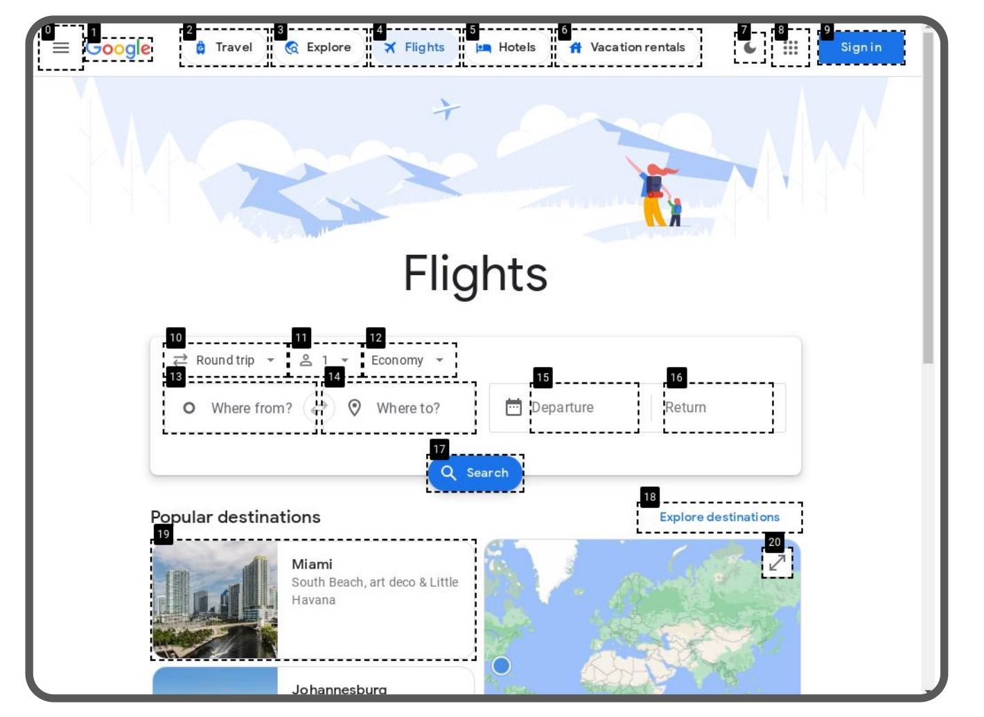
For certain actions, agents need to select a specific element from previously presented marks. When the model decides to click on the Search button from the example in the image above, the output would be: “Click [17]” If the user wants to specify the departure city, the action will require an additional parameter with some text. In this case, the example output might be: “Type [13]; Warsaw”
ReAct prompting – How the Web Agent Thinks and Acts?
The agent employs the ReAct prompting method to carefully consider its actions. ReAct is inspired by how humans naturally combine acting and reasoning to learn and make decisions. Acting allows the agent to interact with external sources, like knowledge bases or environments, to gather additional information. Reasoning helps the agent develop, track, and update action plans, as well as manage exceptions.
WebVoyager uses ReAct in the following way:
Fragment of WebVoyager prompt, source: https://arxiv.org/pdf/2401.13919
This approach can significantly enhance the model’s performance. For instance, consider the deepsense.ai web page shown below. WebVoyager has been assigned the task of navigating to the Services tab. However, through its improved reasoning capabilities, the agent recognizes that it must first close the cookie window to proceed. The output is:
- Observation (from previous step): the image below.
- Thought: To proceed, I need to accept the cookies to interact with the website properly.
- Action: Click [24]
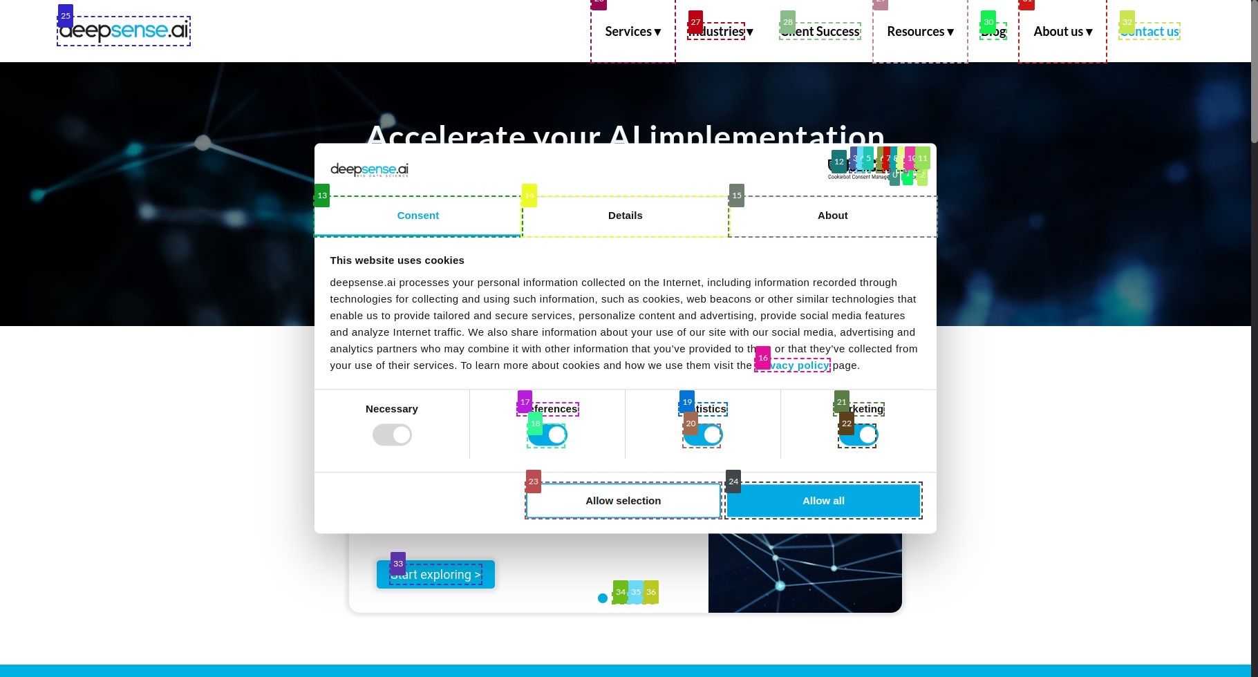
Observation with current web page status, source: https://arxiv.org/pdf/2401.13919
WebVoyager in Action. A Demo
We wanted to see how this agent works in some real-life scenarios. Let’s say that a client wants to get more information about our company. This is how the query looks like:
- “How many commercial projects does deepsense.ai have? You can find that information on their site under the AI Guidance Services tab.”
As you can see, this instruction is quite detailed. Of course, we can also give it a simpler version, but increasing the detail means a greater chance of success.
Whole process can be seen below. The final answer from the model is:
- “deepsense.ai has 200 commercial projects.”
Demo of WebVoyager operation, source: own study
Agent-E: Unleashing Web Automation with LLMs and Compact HTML
In July 2024, just one month after the release of WebVoyager, Emergence AI developed Agent-E, a novel web agent that brings significant advancements over previous state-of-the-art web agents. In this section, we’ll explore how Agent-E works, including its architecture and advanced techniques for processing web content.
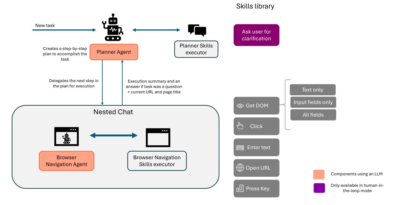
Solution Architecture Overview
Agent-E is designed with a high-level architecture that includes two LLM-powered agents: the Planner Agent and the Browser Navigation Agent, supported by two executor components, the Planner Skills Executor and the Browser Navigation Skills Executor. Each LLM-powered agent has a set of skills, which are Python functions that the LLM can call to perform specific tasks. The executor components are responsible for carrying out the functions that the LLM selects and then reporting the results back to the LLM.
Agent-E task execution flow overview, source: https://arxiv.org/pdf/2407.13032
Agent-E is built using the Autogen framework, which is an open-source tool for creating multi-agent collaborative systems, and Playwright, which handles browser control. The architecture is designed to take advantage of the interaction between these skills and agents.
How Tasks Are Handled with Agent-E
When a user gives a command, Agent-E’s Planner Agent breaks down the task into a series of actionable steps. These steps are then assigned to the Browser Navigation Agent, which is freshly instantiated for each task to ensure that it starts with a clean slate and doesn’t carry over any previous context. This agent uses its foundational skills to assess the browser’s state and control it accordingly, executing the required steps to complete the task.
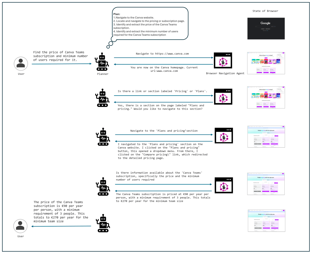
An illustration of Agent-E in action, showcasing the interaction between the planner and the browser navigation agent to complete the task of finding the price and minimum user requirements for a Canva Teams subscription, source: https://arxiv.org/pdf/2407.13032
Agent-E Skills Design: Sensing and Action
Agent-E’s skills are categorised into two main types: Sensing Skills and Action Skills.
- Sensing Skills: These skills enable the Browser Navigation Agent to understand and interpret the webpage using various HTML synthesis techniques. Depending on the task, the agent can extract just the text content, identify input fields, or list all interactive elements on a page. This selective approach helps avoid the pitfalls of dealing with noisy or irrelevant HTML data.
- Action Skills: These skills are designed to perform actions on the webpage, such as clicking a button, and then observe and report any resulting changes. For example, if a click action triggers a popup, the agent reports this change, helping the LLM determine the appropriate follow-up actions.
After executing each skill, the agent provides feedback in natural language, indicating whether the action was successful or not and explaining the reasons behind the outcome. This conversational feedback helps the LLM to better understand and correct any errors, leading to more accurate and efficient task execution.
Agent-E HTML Distillation: Optimising Web Interaction
One of the standout features of Agent-E is its advanced HTML distillation techniques. The size of a webpage’s HTML can significantly impact the speed, cost, and effectiveness of the LLM’s processing. To tackle this, Agent-E compacts and distills the HTML, preserving only the most relevant information for the task at hand. This process is critical because HTML can be so large that they often exceed the context window of an LLM, rendering them impractical for processing in their raw form.
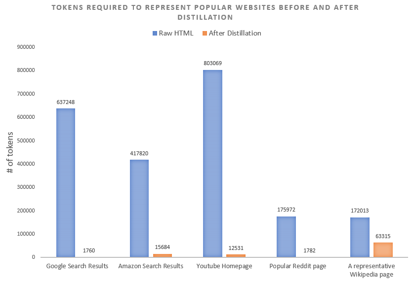
Illustration of the difference in token counts between the raw HTML of popular websites and the more streamlined version after applying our distillation process, source: https://www.emergence.ai/blog/distilling-the-web-for-multi-agent-automation
Agent-E in action. A demo
This demo showcases Agent-E in action. A query, entered into the Agent-E sidebar, asks how many commercial projects deepsense.ai has. Upon submitting the query, Agent-E quickly processes the request, demonstrating its capability to understand complex queries and provide precise guidance. This example illustrates how Agent-E can assist users in navigating websites and retrieving specific information.

Evaluating WebAgents: Beyond Simplification and Toward Real-World Complexity
Assessing the performance of a WebAgent is a complex task. Earlier methods often treated agents like stateful functions, comparing outputs to a reference or ground truth. This approach, relying on keyword or phrase matching, struggled with nuanced or multi-step responses.
Additionally, earlier agent evaluation environments tended to oversimplify real-world tasks, limiting task variety and reducing complexity. These simplified environments often restricted agents to pre-defined states, limiting their ability to explore diverse, dynamic scenarios.
The following sections will introduce a range of new evaluation frameworks, each designed to assess WebAgents on multiple dimensions, including context-awareness, interactivity, and problem-solving strategies, to better reflect their performance in complex environments.
WebArena: Advancing Agent Development with Realistic Web Complexity
A new wave of WebAgent benchmarks has emerged to push the boundaries of autonomous agents in real-world web environments. One noteworthy example is WebArena that offers a realistic setting with four operational web applications across domains: online shopping, discussion forums, collaborative development, and business content management. WebArena includes utility tools such as a map, calculator, and scratchpad, allowing agents to mimic human-like interactions with web content. It is also supported by a broad range of knowledge resources, from general information like Wikipedia to specialized manuals for tools integrated within the system.
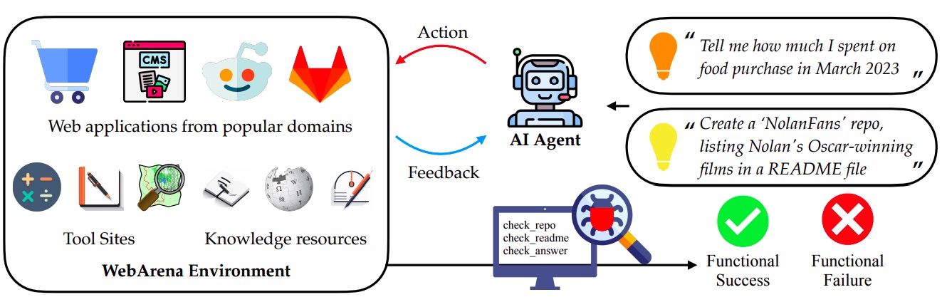
WebArena benchmark features 812 tasks evaluated using metrics such as Exact Match, Must Include, and Fuzzy Match, focusing on outcomes rather than steps. In tasks related to site navigation or content manipulation, WebArena assesses performance by programmatically examining the intermediate states during task execution. This process verifies whether the agent is interacting correctly with the website or database at each step. Additionally, agents are tested on their ability to recognize unachievable tasks.
WebVoyager Evaluation: Embracing Real-World Web Diversity
Another benchmark, introduced in the WebVoyager paper, focuses on evaluating agents in more dynamic, real-world scenarios. It spans 15 websites that represent various aspects of daily life, from online shopping and education to collaborative platforms and real-time information sources. Task generation in this system is a hybrid approach, combining automated processes with human validation to ensure diversity and accuracy. The final dataset consists of 643 tasks, including both well-structured queries and open-ended tasks like summarization.
A key feature of WebVoyager is its dual approach to answer annotation. For tasks requiring stable, factual responses, it uses “Golden” answers. For more open-ended or dynamic queries, it allows for multiple valid responses with “Possible” answers, reflecting the nuanced nature of real-world web interactions. This flexible evaluation system ensures that agents are not just judged by rigid correctness but by their ability to provide feasible, high-quality solutions.
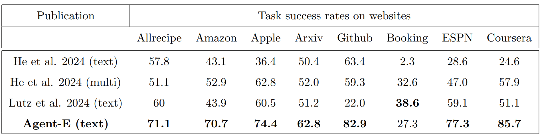
Agent-E: Introducing Metrics for Evaluating Task Efficiency and Resource Utilization
Adding to this landscape, Agent-E introduces four key metrics for a comprehensive evaluation of web agents:
- Task success rates measure the percentage of tasks completed successfully across various websites.
- Self-aware vs. Oblivious failure rates differentiate between failures where the agent acknowledges its limitations and those where it provides incorrect answers or actions, with self-awareness being critical for minimizing errors.
- Task completion times capture the average duration required to complete tasks, regardless of success.
- Total number of LLM calls counts the average number of calls made by the agent (both planner and browser navigation) during task execution, reflecting its efficiency and resource utilization.
Navigating Limitations in Real-World Applications
Web agents show promise but face key challenges limiting their real-world use. Replicating complex web actions, like precise dragging motions on web pages, present difficulties due to their continuous nature. File compatibility is also an issue, as agents like WebVoyager can only handle basic file types such as text and PDFs, but struggle with multimedia formats like video, limiting their versatility.
Open-source models face trade-offs between image resolution and context size, hindering detailed web navigation. The need to integrate both text and visual inputs is also critical. Agents must integrate text and visual inputs to improve performance on visually complex sites, like booking systems or travel platforms, where calendars and intricate visual components are involved.
Finally, a “human-in-the-loop” approach is crucial for ensuring accuracy and managing security risks, while balancing ethical concerns and environmental costs. The authors of Agent-E stress that human-in-the-loop workflows are critical for the adoption of agentic systems, although no benchmarks currently exist for such agents.
The Future of Web Agents and Web Automation
Despite recent breakthroughs, we are still at the early stages of the evolution of Web Agents (and LLM Agents in general). The future promises many intriguing advancements, offering much to explore.
Currently, Agent-E focuses on textual input, while WebVoyager specializes in visual data. A unified approach that combines both could provide a more comprehensive understanding of web environments. This convergence of textual and visual inputs (and perhaps other modalities like audio or video) will allow agents to grasp context more holistically, resulting in more accurate and effective responses.
Present-day solutions, though fascinating, are still the products of research environments and are not yet ready for production use – a lot of unexpected things can happen like infinite loops, bad action parsing etc. In the future, agents will become more robust, addressing most edge cases and mitigating the non-deterministic nature of language models as much as possible. To achieve this, substantial input from software engineers is necessary to make these systems production-ready.
As an AI community, we have to work hard to introduce better methodologies for measuring agent performance. With an increasing number of testing methods and datasets, we will be able to conduct more extensive evaluations and identify specific areas needing improvement.
Summary
In conclusion, the journey of Web Agents from simple web scraping tools to sophisticated systems like WebVoyager, and Agent-E showcases the immense potential of leveraging large language models for web automation. Despite significant advancements, current Web Agents still face hurdles such as handling complex interactions, integrating multimodal inputs, and ensuring precise task execution in dynamic web environments. Addressing these challenges requires continuous innovation and development, along with robust evaluation frameworks to ensure real-world applicability. With these improvements, Web Agents could significantly enhance our ability to efficiently and effectively navigate the complexities of the web.