

When large language models come into play as part of building a competitive advantage within services or products, many additional questions arise. Effective implementation that brings real business value requires the analysis of aspects such as reliability, high availability, security, data privacy and many more. Such research is time-consuming, which is why deepsense.ai comes with some of it done for you already.
For the purposes of our projects, we have reviewed the key aspects related to the use of OpenAI models. In this article, we share our insights related to two main ways of accessing the OpenAI models, both directly from the organization’s API and via Microsoft Azure OpenAI Service. We review the two options for the central block of this kind of platform that can be covered by the services offered by the two.
OpenAI is an artificial intelligence company founded in December 2015. Its influence in terms of making AI available to a large community of users and becoming part of pop culture has been nothing short of spectacular. Each series of their famous GPT models quickly became popular, giving rise to excitement, doubts, concerns, and… new business opportunities!
The partnership between OpenAI and Microsoft dates back to November 2021, and it seems that their common goal and a shared ambition to responsibly advance cutting-edge AI research and democratize AI as a new technology platform only strengthens this collaboration. Microsoft is one of the biggest public cloud providers. Their immense cloud resources and robust services have supported OpenAI research in their collaboration, but are not limited only to that company. Currently Microsoft offers resources to other Azure users, allowing them to benefit from the results of the cooperation with OpenAI within a well-known, mature and safe cloud environment.
OpenAI has released a simple and intuitive API to interact with their models. The requests are handled by OpenAI servers. Such an approach allows us to focus the team’s efforts on research rather than infrastructure and computing challenges. The models were developed as a text in, text out interface based on text prompts. The pattern provided in the request decides. The API and Python SDK openai package can be used.
As far as data security is concerned, the situation changed in April 2023. OpenAI ChatGPT had received heavy criticism from both users and experts concerning its further data usage and retention policies. Currently it is easier to ensure data are not being used to train the models by default. The OpenAI blog confirms that, having chosen to disable history for ChatGPT, new conversations are going to be retained for 30 days before permanent deletion only for monitoring abuse. The TLS communication of OpenAI API allows for in-transit encryption for customer-to-OpenAI requests and responses.
From the perspective of Microsoft Azure, having the early feedback lessons from people who are pushing the envelope and are on the cutting edge of this gives us a great deal of insight into and a head start on what is going to be needed as this infrastructure moves forward. Microsoft currently provides exciting offers that combine the main advantages of the two parties via Microsoft Azure OpenAI Service.
As we can read in the article by Eric Boyd, Corporate Vice President, AI Platform: The power of large-scale generative AI models with the enterprise promises customers have come to expect from our Azure cloud. The service enables the customers to run the same models as OpenAI, benefiting from the enterprise-scale features of the Azure cloud.
In terms of data security, apart from private networking and regional availability, Azure provides privacy and confidentiality when one entrusts them with data. Azure fulfills the following expectations:
To sum up, if you need to ensure no further usage of your data, Microsoft, as a provider, creates a safe place for your data. If you already possess any data on Azure servers, the choice of service is low-hanging fruit. Additionally, their safety will not be affected in Azure OpenAI Service. As this is a very explicit declaration about safety, we recommend using this service especially when data vulnerability is of concern.
There are several engines (corresponding to the models) as their capabilities (and customization opportunities through fine-tuning) differ. For both OpenAI API and Azure, there are a few categories of models which are ready-to-use or allow zero- or few-shot learning depending on the use case. One can always choose between alternative categories:
The models released by OpenAI have been organized into series corresponding to experiments and the respective tasks the engines perform and the engine categories listed above partially overlap with the series but represent a different quality.
Although one can find the entire list of models accessible via OpenAI API in their docs, we are going to limit our attention to the models that are also available in the Azure OpenAI service. Shortly, we will skip the Dall-E, Whisper, Moderation and some GPT-3.5 series models – they are not explicitly accessible in the latter service and are beyond the scope of this related post summarizing aspects of LLM API usage. We compare the context length and time range of the training data set (the maximum number of tokens if approximated to thousands). The details of the models are far beyond the scope of this post, yet we want to provide the basic intuition behind the engines that can be used.
The GPT-3 base models available are Ada, Babbage, Curie and Davinci – the ordering is not accidental and represents the capability vs speed trade-off with Ada as the fastest engine and Davinci as the most powerful. All models were trained on data from up to October 2019 and have a maximum of 2k tokens.
Even though all GPT-3 based engines are usually substituted with the more powerful GPT-3.5 series model, they are also served by fine-tuned alternatives (text prefix) and are available for embedding tasks or are fine-tunable with user data.
For Azure OpenAI Service, these are the models available for getting embeddings. The same holds true for OpenAI, but they also recommend a second generation embedding model, text-embedding-ada-002 (8k tokens) designed to replace the previous generation of embedding models at significantly lower cost.
If one is interested in a modern series of language models optimized for chat but suitable for traditional completion tasks as well, there are at least two served by both providers. The GPT-3.5 series has a flagship model gpt-3.5-turbo (4k tokens) – it is recommended as a cost-effective and the most capable model. Please take into account the fact that, though OpenAI API supports multiple countries (without explicitly mentioning the server regions) not all regions of Azure OpenAI Service enable this engine (for example Central US, in contrast to Eastern US or Western Europe).
Another alternative is GPT-4 of an even higher series that has recently aroused the interest of the public. At the time of writing, it is available in the API documentation as limited beta. In the case of this engine, the regional support in Azure is narrowed down to the Eastern and South Central regions in the case of the US and is not available in other regions. One should consider the fact that currently there is a waitlist to join to get access to this engine API in Open API. This engine is a large multimodal model with 8k and 32k maximum token variants and is meant to solve difficult problems and perform with advanced reasoning capabilities and provide results at a greater level of accuracy compared to the previous models thanks to its broad general knowledge.
The situation with LLMs understanding and generating code changed in March 2023. For users who are interested in using the engines that were commonly used, namely the code-davinci and code-cushman models (8k and 2k tokens respectively and the speed advantage of the latter), they are still available in Azure OpenAI Service. The same engines are deprecated in OpenAI API and the chat models are recommended for the task – the capabilities remain similar..
Having discussed the details of the various models above, we present a table to summarize the high-level specifications of the models.
| Series | Latest model | Max tokens (by 1.024) | Training data |
| GPT-3 | davinci | 2k | Up to Oct 2019 |
| curie | |||
| babbage | |||
| ada | |||
| code-cushman | N/A | ||
| code-davinci-001 | 8k | Up to Jun 2021 | |
| GPT-3.5 | text-davinci-002 | 4k | |
| gpt-3.5-turbo(-*) | 4k | Up to Sep 2021 | |
| GPT-4 | gpt-4(-*) | 8k, 32k | Up to Sep 2021 |
Table 1. OpenAI model sizes and training data overview. Source: OpenAI docs.
At this point in our analysis, it is worth mentioning two main similarities.
Co-development of the APIs with OpenAI and ensuring compatibility to make the transition and integration of the models seamless is the strategy behind Microsoft Azure OpenAI Service. Thus, switching between both services should be fairly easy and might simply involve an alternative configuration to your codebase. If the business use-case and cost optimization strategy is suitable, dynamic migration between providers comes into play.
OpenAI claims that the models may encode social biases (negative sentiment towards certain groups/stereotypes). These issues are addressable for each provider but in a different manner (please see the section about differences). Moreover, the models lack knowledge of events which took place after August 2020.
In addition to the characteristics of both solutions already described in this article, it is worth noting three basic differences.
Pricing is one of the key differences between the providers. The Microsoft Azure calculator helps to estimate pricing of fine-tuning, as well as hosting a fine-tuned model, whereas with OpenAI API one is charged only for the tokens used in requests to that model. The pricing of single API requests (per 1k tokens) of both providers is alike..
Based on the OpenAI API usage policies, all customer data is processed and stored in the US. If the volume of your data is large enough, it is recommended to keeping the compute power close to the data in order to avoid moving it excessively is recommended, so as to avoid network transit overhead. This seems to suggest that the choice of Azure OpenAI Service would be best if you need elasticity or a particular region of availability.
From the perspective of an Azure OpenAI Service user, the recommended text-embedding-ada-002 model is available in Azure OpenAI, but the number of tokens used might be limited (see this thread).
The model used with OpenAI API can be supported with their Moderation model to classify and prevent content that is hateful, harmful, violent, sexual or discriminates against minorities. Put simply, it must be compliant with the usage policies of OpenAI. Similarly, the content requirements must be met in the case of its Azure counterpart, so the content policies are intended to improve the safety of the platform for both the input and output of the engines, and are always explicitly filtered.
For more information, see and compare the OpenAI safety standards and the Azure service Responsible AI section in the docs.
A multitude of available models allow for various implementations for your services or products and provide a dynamic approach to scaling and optimizing costs and performance. The adoption of OpenAI solutions creates exciting new business opportunities for various industries. On the other hand, there is an exciting world of alternatives, and our experts can guide you on your journey. Let us know if our AI development agency can help build your vision incorporating large language models!
Recent breakthroughs in AI have showcased the vast potential of convenient natural language interfaces and taken the web by storm. Many companies across various verticals have started looking for specific business use cases to implement this technology. As our motto is “There is no better way to show our capabilities than to build solutions”, we have developed various technical showcase implementations to inspire and present potential solutions. In this blogpost we will discuss our latest GPT-based solution addressing the challenge of extracting knowledge from a set of PDF documents.
Meet Niffler

We have given our project the codename ”Niffler”. The name was inspired by a magical beast from the Harry Potter universe which is attracted to shiny things. We used AI to create its mascot image (see the result above!). Niffler’s task is to digest user-provided PDF (or text) documents and provide a chat interface along with highlights of the relevant document. Development of the application enabled us to put our experience into practice.
At any point in time, each company generates a huge number of documents – from legal, finance and administrative documentation to knowledge databases pertaining to internal processes. Employees join or leave the company, projects finish up, others start, and the pile of documents continues to grow. At some point, keeping track of what was done and where to find the information is impossible, and many hours are wasted. If the company’s core business is not about document organization, it represents a cost sink which is hard to even measure.
In some cases, even if the right document is found, it is often not enough – the document can be too long to read properly, or the need to supplement it with other ones to gain relevant insight arises. Hiring a dedicated staff member to search for information can be a possible solution, but wouldn’t it be great if an application could read all the documents, find and match relevant information and then provide a concise answer with all the required references? If we combine this idea with another AI model for speech-to-text, any team at a company could access technology similar to that owned by the superhero Tony Stark and efficiently work with the company or external data, which will of course provide a competitive advantage.
The business challenge for Niffler was described in bullet point form:
Our core technology is independent of the source of the GPT model, as we don’t want to be vendor locked, but rather flexible for every potential need. We decided to use OpenAI as an external component as it suited our needs best.
In order for Niffler to start working and supporting us in our daily work related to document analysis in accordance with the above-mentioned assumptions, we had to consider various crucial aspects, which we discuss below.
Operation costs for a GPT-based application
As with all projects, the costs depend on the choice of the model and where it is used. For example, in the case of OpenAI API payment depends on the number of tokens required by an input and output (neural networks require input paragraphs and sentences split into small processable units called tokens), but on the other hand Azure charges by the inference time, counting how many minutes your requests take.
A great way to see what a token is would be to visit the OpenAI tokenizer page which graphically displays it for your text.
One important detail is that the number of tokens includes not only direct user input but also hints we need to pass to the network – such hints provide additional guides, context or examples which are necessary for better results. Such techniques are called zero-shot and few-shot learning and provide a way to better align outcomes with expected results for concrete tasks without the associated costs of training a specialized model. There is also a hard limit on the maximum number of tokens acceptable to the network; the bigger the network, the more it can take as an input.
You may wonder about a specific example of why there is a need to have additional context provided to the network, as of course it increases operational costs. Please note that the model does not have a memory of a conversation (it cannot remember anything that either a user or the model itself wrote a second ago!) and to help it remember, it is necessary to inject the chat history or just a summary of it. The presence of additional, specially formatted prompts can enforce consistency and quality – it is a technique to prevent answering outside the desired bounds and to ensure it acts appropriately, even for a malicious user.
Moderation of AI
It is an unfortunate fact that large language models can generate outputs that are untruthful, toxic or simply unhelpful, and special care is required to address that issue. Providers of services like OpenAI and Azure provide some black-box moderation – but that’s not enough. To address such concerns, we came up with and implemented several techniques – one of which is to add an additional AI layer to moderate output. More details about our design are described in the reliability and security section later in the article.
We started with a proof of concept prototype – its main goal was to get feedback and iterate fast on the idea. We used Streamlit, a library for quickly building graphical interfaces for data science projects – it does not allow a high level of customization, but it allows you to quickly present visual results which greatly simplifies communication, especially with less technically-oriented people. Additionally, a major plus point is that it is easy for a data scientist to use without the need to involve frontend and backend developers.
The video below shows a set of prototype features of our AI system:
The prototype has more features than our polished demo application and it is a teaser of what we can do.
Video 1. Prototype flow: We started by searching a set of documents and then asking for more details focused on those found. We also integrated a Bing search allowing the model to dynamically fetch data from the internet as requested.
The prototype allowed us to experiment with many different ideas before settling on a set of features to focus on. It also improved communication with project stakeholders, but even more importantly each team member showcased their work post daily with other team members which greatly improved internal collaboration and made it more fun.
At the time of writing, out-of-the-box GPT-like models are unable to process big chunks of data or work with standard documents like PDF or Word documents.
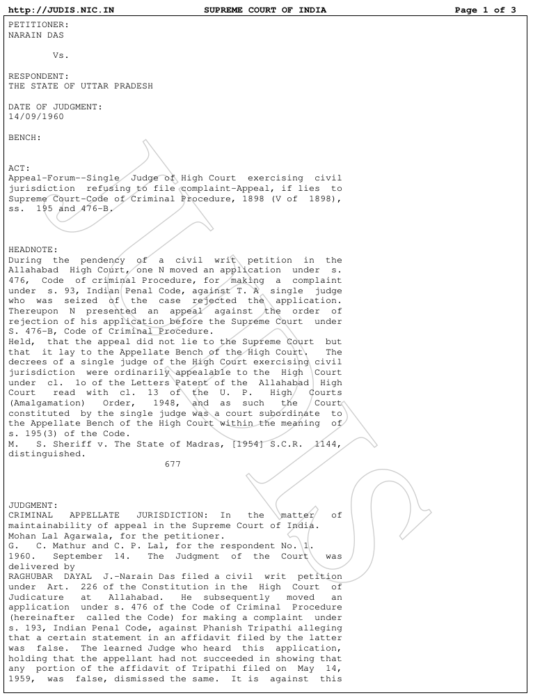
Figure 1. Example of a PDF legal document we used for our tests from this Kaggle dataset Indian supreme court judgment.
To solve this challenge, we created a dedicated preprocessing step which digests native PDF formats – parsing PDF in general is not an easy task and OCR might not always work so well, but for the purposes of our prototype it is sufficient.
The resulting canonical form is then passed to an intelligence processing block – AI reads chunks of text, creating a summary and tags to make efficient searches possible – which calculates so-called embedding vectors. They encode semantic information in a very efficient manner. Such vectors are then stored in the vector database along with additional metadata.
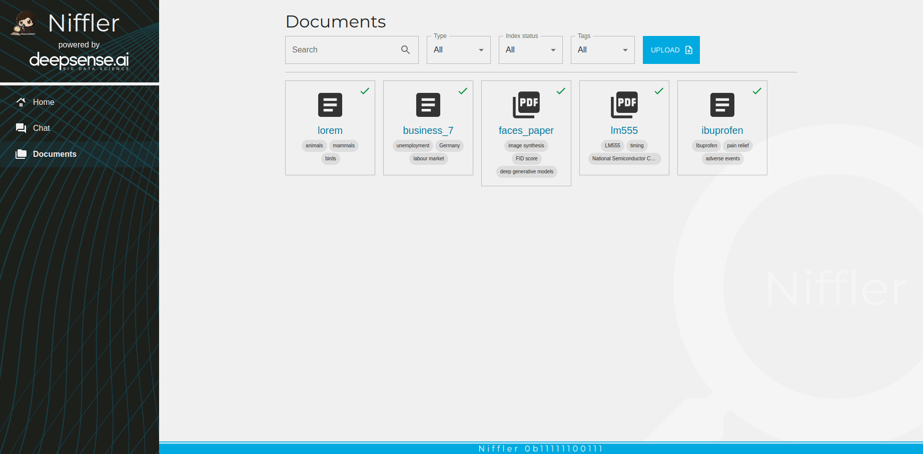
Figure 2. Each uploaded document has 3 tags useful for searching, clustering and prompt tuning.
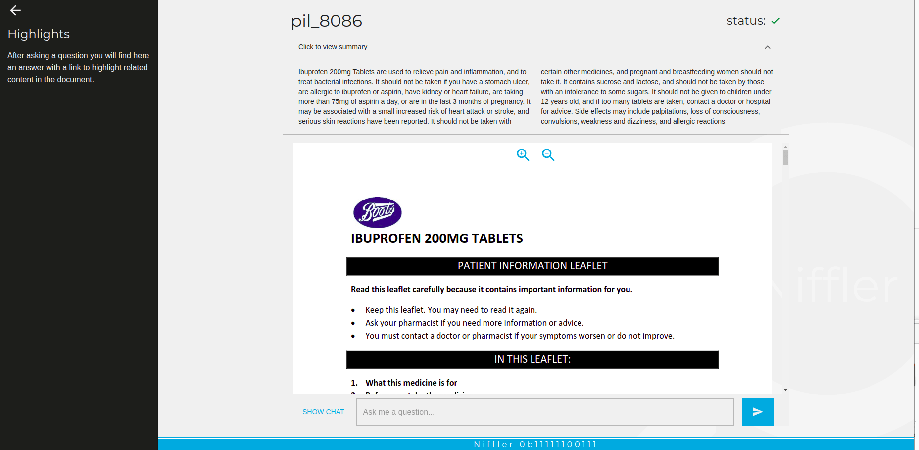
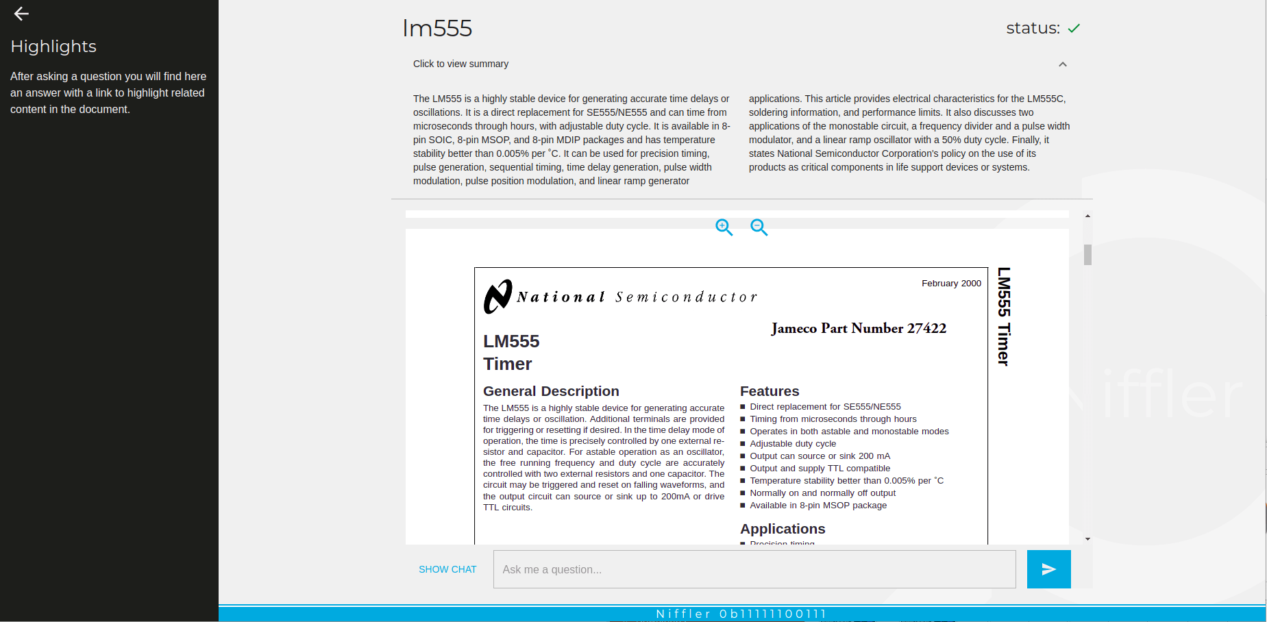
Figure 3. Two distinct PDF documents with summaries generated by AI. The shorter form is a great way to quickly learn about the content, as well as to align the system to focus only on questions and answers related to the document context.
This is a one-time cost to include each document in a database and it does take some time – however, the database can then be extended easily on the fly to include new documents, which can be done in the background without stopping the system from functioning.
This approach provides additional control which can be useful when it comes to improving or extending the performance of the system.
Software should be pleasant to use. To achieve this, we decided to build our frontend as a ChatGPT-inspired interface – familiarity with chat interfaces makes it very easy and natural to use.
We have prepared two main views – a standard chat and document preview, together with a left sidebar which contains highlights, or questions with answers, serving as links which allow a user to revisit previous and current selection in the source document.
Screenshots, of course, are not enough to present interaction, so we decided to record a set of short clips to capture the user experience. One major strength of our application is that a user can not only quickly revisit answers, but also jump with just one click to the relevant source information and validate whether AI has done a good job with the answer provided.
Video 2. Question about a court case and inspecting the full document to show that only a small, relevant portion is highlighted.
Video 3. Medical leaflet – one question asked.
Video 4. Medical leaflet again, with more questions and a showcase of the highlights.
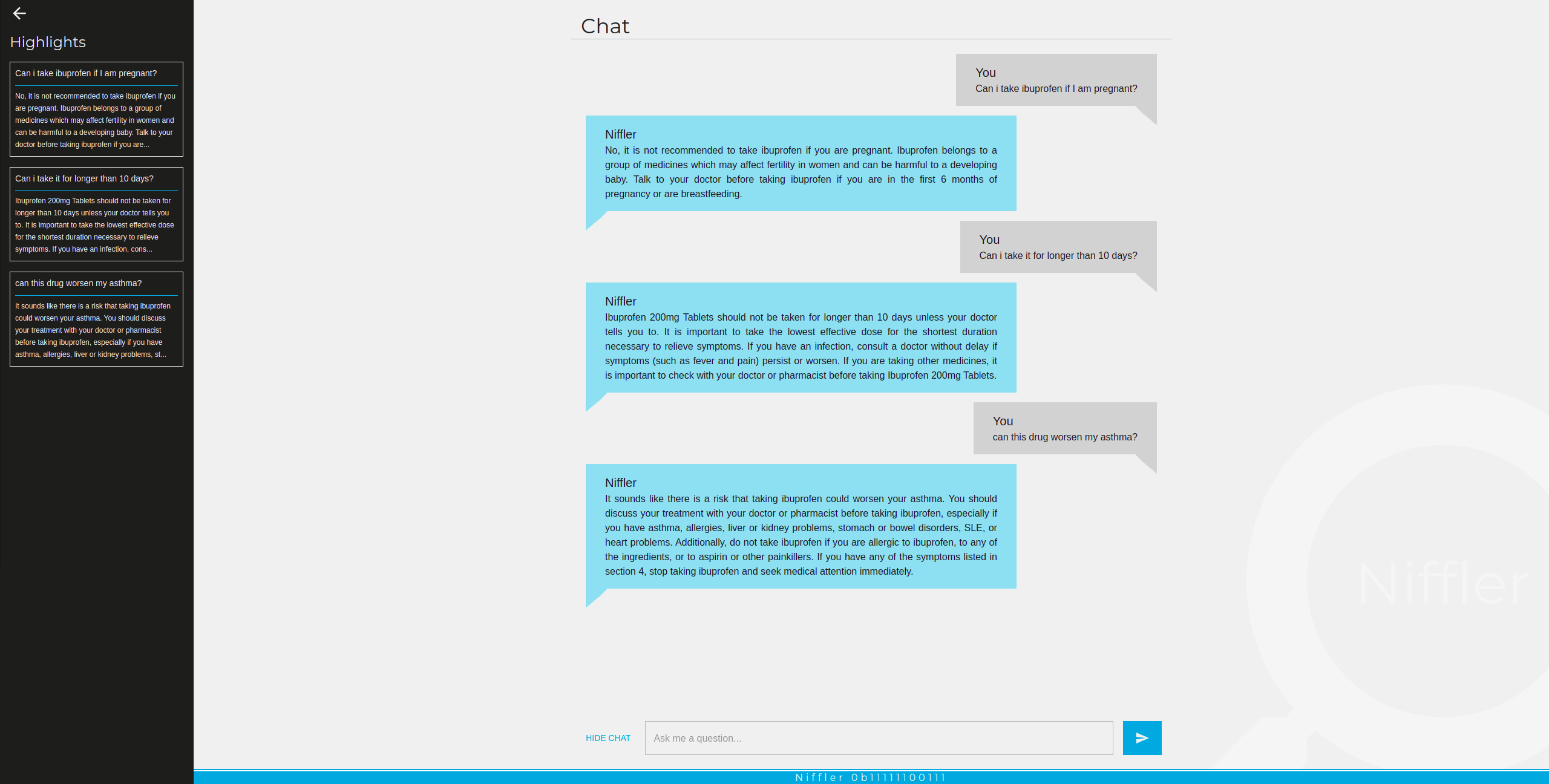
Figure 4. Example chat. Please note that our application is language-agnostic as the underlying GPT model.
GPT models can return different answers when asked the same question multiple times and there is no formal guarantee that they won’t make mistakes, answer on topic, or even offend a user. Indeed, it is a challenge many have experienced; it is mentioned in the Bloomberg article, the official limitations of GPT-4 (the most powerful model), and it is easy to find more articles on the topic. A mitigating solution that seems to work quite reliably for our use case is the additional 3 steps for standard flow that we describe in more detail below.
Our first line of defense is the aforementioned built-in moderation from OpenAI. We also researched prompts to ensure that AI can only provide answers on selected, narrow topics and data. The input prompt to the model is built only with the context connected to the question given the automatically generated document summary and 3 tags for a given document. Dynamic prompt engineering yields better results than a generic prompt and is a great alternative to manually hand-crafted prompts.
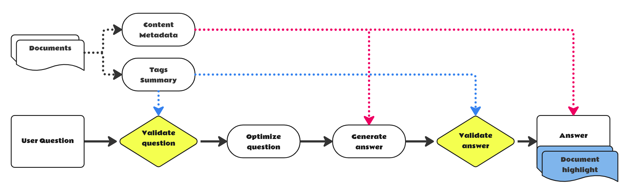
Figure 5. Simplified flow for a single document interactive question and the answers we have implemented.
The third line is actually our secret sauce – we use another AI to moderate output.
We tried several attacks by injecting text prompts known to alter model behavior (asking it to act as someone else and other different kinds of persuasions, DAN etc. which are mentioned by people on Twitter) or try to get it to answer something unrelated or on the topic but possibly harmful. We have failed to break it so far. On the other hand, it also sometimes leads to it not answering questions if they are not really on the topic. Depending on the use case, we can tune it to be more or less restrictive as all additional checks are opt-in. We also found out that even if the model refuses to provide an answer, the highlights mentioned in the next paragraph might be returned correctly.
To complete the user experience, we also quoted and showed what the source of information provided by Niffler is. This feature is a major selling point of our approach for any user as it addresses 2 aspects – verification of AI model output by the user and efficient information search. We especially placed a great deal of emphasis on presenting minimal, raw text in a visual way in the source document to enable the user to save as much time required to read the original content as possible. A concise AI answer is an added extra, not a replacement for your data source. At the moment truthful, fact-based answers and links to source information are still an unsolved problem under active research. Addressing this issue is very challenging, but we have already seen some promising results and gained a number of key insights during the development phase.
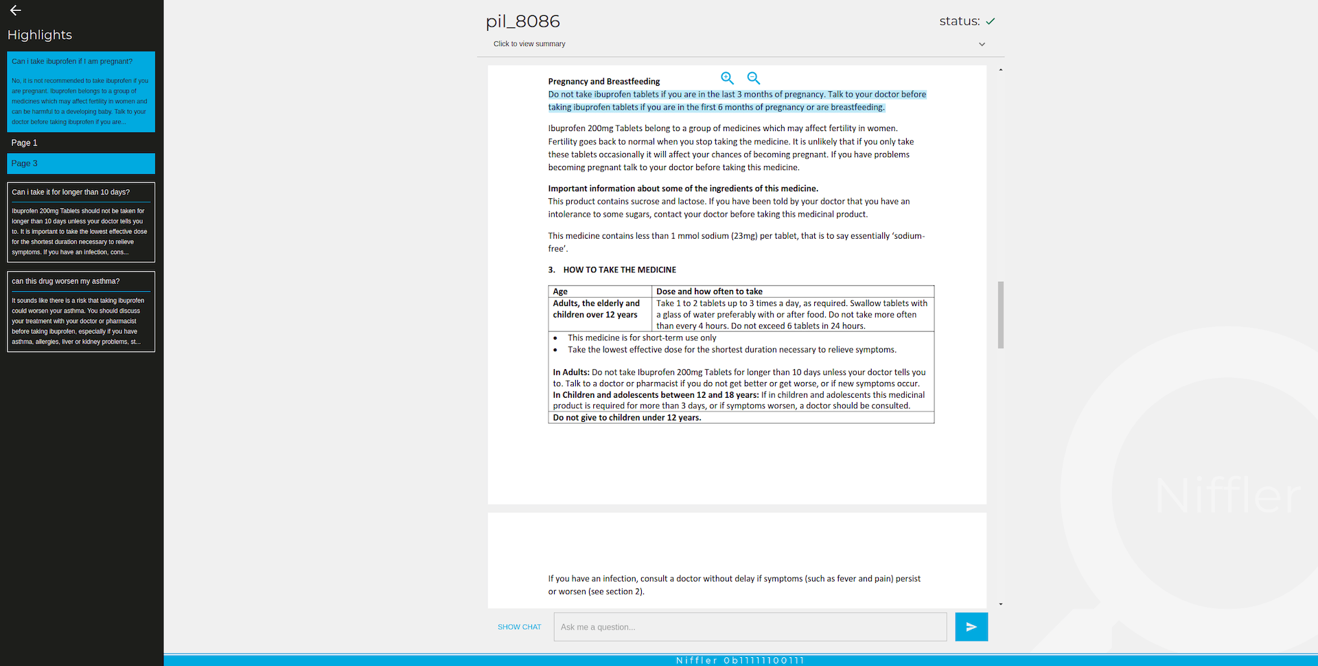
Figure 6. Example of an answer with the citation selected – in the PDF file we highlight the exact sources of information used by GPT, allowing a user to focus only on short, concise and important information.
We have built a useful and interesting application – we hosted it internally on our servers and made it available for deepsense.ai employees to use. Our highlight module is one of the key strong points and people found it very useful. External use cases for the current Niffler version we witnessed included information retrieval from research papers and device manuals. Additionally, we created a knowledge base which we have shared internally (for now) with our colleagues to propagate everything we have learned.
As we thrive on excellence, there are still more things to do.
Static knowledge is not enough for the rapid changes that are happening in the world of AI. That is why we added the possibility of integrating with external sources of data such as SQL databases or any APIs to Niffler. For example, if we would like to do an analysis of our competitors, we could search for different types of data along with recent business analyses, stock prices and so on.
Moreover, we created a prototype mode of an AI agent who can search and scour the Internet on its own.
On top of that, one of our team members set up an integrated Whisper service (a speech-to-text model API provided by OpenAI) – why does someone need to type on a keyboard if a superhero can just say things? With real-time transcription and text-to-speech synthesis, we make it even more enjoyable to use. Imagine being able to search for your Q3 financial statistics and receive them directly to your ear during a conversation with stakeholders! You could eliminate the need for someone to look it up and prepare a report.
Such things are entering the realm of possibility, and likely only companies which understand and can use such potential will dominate the market.
If you are interested in your own solution, feel free to let us know! We can help you to build a competitive advantage by adding the features of GPT and other LLMs to your products and services.

1. Introduction
2. Experimental setup
3. Questions and empirical answers
4. Summary
5. Appendix – Diversity calculation
In previous blog posts, we introduced you to the world of diffusion models. We also proposed an evaluation method for various aspects of generative models based on the example domain of face generation. We now use the previously introduced metrics imitating human-like assessment. By combining theoretical concepts and empirical experimentation, we aim to provide comprehensive and evidence-based answers to the hidden questions that often arise in the fine-tuning of these models. The specific domain we have selected is personalized face image generation, but the conclusions and methodology are applicable elsewhere as well. So get ready to explore the world of stable diffusion from a unique perspective as we share our insights and findings using the methods we’ve developed!
It is essential to grasp the core of our research before moving forward. Here, we provide a condensed glimpse into our objectives, the data we analyze, our approach to prompt engineering, and the computational power propelling our discoveries.
The generation of a specific class of images using diffusion models capable of a broader range of expressions is a common scenario. To reflect this, we chose the generation of personalized 512×512 images of faces as a particular subdomain. The aim here is to optimize:
With those goals in mind, we wish to provide some answers to the following questions:
In this subsection, we will peel back the curtain and reveal the essential components of our experiments. We will provide an in-depth look at the data we employed, the hardware that powered our endeavors, the intricacies of prompt engineering, and the metrics used to evaluate the performance of the model.
While diffusion models can generate practically any image, one is usually interested in a specific domain with intrinsic quality criteria. As an example domain in which to test our empirical methods, we chose personalized portrait generation. The choice was a very conscious one. Portrait generation is popular; quality assessment is intuitive and requires no experience; several partial, domain-specific metrics are easy to conceptualize (similarity to a given person, aesthetic quality, etc.); and the conclusions may translate well to other domains.
To hone in on the intricacies of diffusion model-based facial image generation, we created a photo portrait input dataset including:
This selection ensured relative diversity and representativeness. Based on this, portrait generation proved a fruitful environment for investigating the capabilities of diffusion models in terms of generating realistic and diverse samples, allowing us to shed some light on the general properties of diffusion models.
Now, a few words about the hardware that allowed us to breathe some life into our models and data, and to perform the experiments.
Stable Diffusion, in its basic form, requires about 40 GB of VRAM to train. With some optimizations, the most ‘inclusive’ setup on which we run DreamBooth finetuning was RTX 2080 Ti, with 12GB of VRAM. We utilized four such GPUs.
We took advantage of various optimizations to achieve this. They included an 8-bit Adam optimizer, gradient checkpointing, and caching images already embedded in latent space. These optimizations helped us manage memory usage effectively, enabling us to work around the limitations.
Prompt engineering is a crucial aspect of our experiments, as it sets the stage for generating meaningful outputs from diffusion.
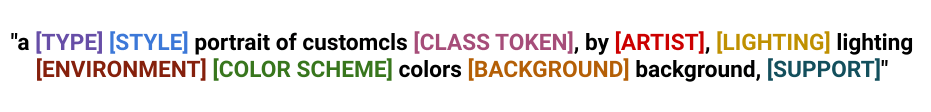
Caption: Our prompt template
We used this template to generate a diverse and robust set of 5000 prompts by randomly replacing prompt components with their corresponding values (see table below). The word “customcls” contained in the template is a token of the object we fine-tune for, while CLASS TOKEN is the ‘base object’, i.e. a similar object already present in the domain before fine-tuning (in our, either “man” or “woman”).

Caption: Table with phrases used to fill the prompt template
We utilized these 5000 prompts during the inference experiments to generate images and assess the performance of any diffusion model. In the training validation process, we carefully selected a subset of 100 prompts and used it at intervals during the training procedures. This allowed us to craft representative input sets and achieve controlled, interpretable results within a reasonable timeframe.
Evaluation metrics are a critical but problematic element of generative model assessment. In our previous blog post, we introduced and evaluated similarity and aesthetics metrics. We encourage you to check it out in detail. In addition to these two metrics, there is another crucial indicator of model quality, namely output diversity.
In the literature, the FID Score is often used for similar purposes, as a state-of-the-art method. Simply put, the FID Score assumes that the model’s training dataset and output set are normal distributions and measures the distance between them. We opted to modify this approach slightly, as we are only interested in the diversity of the model’s generation after fine-tuning, not its comparisons with either the (tiny) fine-tuning or (huge) pre-training dataset. Our diversity assessment directly measures variation in the generated image sets during evaluation. When tracking diversity, we want to ensure that the variety of images produced by the model does not decrease significantly from the base value at the starting point. A detailed description of how we calculate the output diversity is described in the Appendix.
By measuring the metric dynamics during the training, we can track the model’s performance and check that the quality of the generated images does not degrade over time.
After we calculated all the metrics for all the relevant images, we scaled them to ranges allowing for the best presentation of the differences that occurred. The assumed min-max metric value ranges are:
Having discussed the technicalities, we can address some of the most pressing questions related to the parametrization of diffusion models and provide answers backed by data and empirical analysis.
We decided to present our observations accompanied by fully interactive graphs to allow the reader to explore the data and draw his own conclusions.
Our data presentation follows our experimental method, and includes these steps:
The first chart shows the dynamics of fine-tuning runs. Based on the metric changes, one can make a number of hypotheses and observations:
If the metrics can signal the breaking point in training, it may be a good sign that it’s time to stop. Since we monitor multiple competing performance dimensions (metrics), different tradeoffs between similarity, aesthetics, and diversity are possible. To accommodate this, we provided weights for each metric. You can use it to adjust the optimal/stop points to your preferences (we used our preferred weights as a starting point).
This way, we can also verify various popular rules of thumb. One well-known heuristic states that the optimal number of steps is 100 * the number of input images. It seems close to the truth, but other options may possibly work better (note that values may change slightly for your metric weights):
Let’s try to use this approach to answer another question that has long troubled the community involved in generative art: what is the influence of the number of input images on the quality of the output?
Instead of focusing on the training dynamics, the graph below inspects a direct relationship between the number of images and the metric values at the final/optimal point of the training. We can see that:
It is no surprise that Stable Diffusion versions 2.0 and 2.1 are capable of significantly better generation than 1.5.
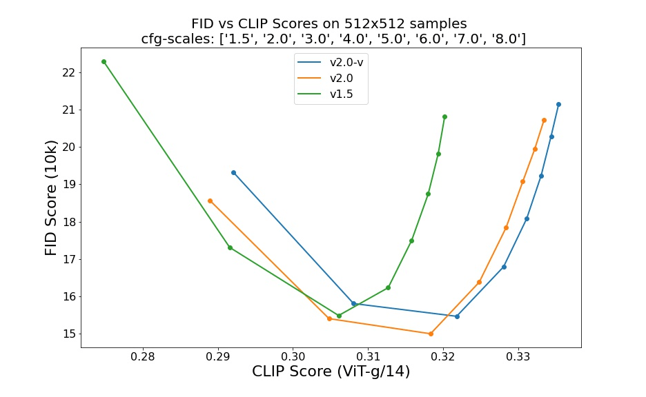
Caption: Comparison of SDv2.0 and SDv1.5 [Source]
While verifying our findings and searching the Internet we found mixed user feedback on Dreambooth + SD 2.0/1 and many similar observations that the 2.0 and 2.1 models are more difficult to fine-tune and it is much harder to generate art-style images with them.
We tried several things, including the use of different schedulers, and switching the encoder to OpenCLIP (used for training versions greater than 2.0). None of our attempts came close to the results from fine-tuning version 1.5. We are not saying that it is not possible, but you may wish to take this into account.
Note: the model weights we used in the comparison were pre-trained on 512×512 images to maintain the reliability of the comparison. It is not out of the question that SD 2.0 and 2.1 models pre-trained on higher-resolution images would have done better.
Thanks to our schematic approach to prompt engineering, we were also able to assess the individual parts of prompts in terms of the quality of pictures they produce. The results are presented after averaging 400,000 generations.
Different parts of the prompt have a specific impact on its quality; we hope that with this analysis you will be able to create better prompts!
Some of the useful insights regarding this analysis are:
In this blog post, we empirically investigated image generation using diffusion models. Imitating human evaluation, we objectively measured aspects usually left to subjective manual checks and arbitrary decisions. We carefully curated a diverse and representative dataset and a relevant prompt base (using a universal prompt template) to facilitate this investigation. Based on hours of experiments and proposed metrics, we investigated the data visually, gained a great deal of insight, and answered key questions concerning the quality of the generated images. You can use our findings in your facial image generations, and our approach can be used as inspiration and extended to other domains.
Let’s denote \(S\) as the set of generated images in a specific evaluation step by a specific model, represented by a set of n-dimensional embeddings.
The diversity measure considers each element of the set in relation to the other elements in the set. In other words, for each \(s_{i} \in S\) comparisons are made with each element of the set \(S’_{i} = S / s_{i}\). The following mean value is calculated for each element \(s_{i}\):
$$
\forall s_{i} \in S \quad d(s_{i})=\dfrac{\sum\limits_{e \in S’_{i}} D_{c}(s_{i}, e)}{|S’_{i}|}
$$
Where \(D_{c}\) is a cosine distance. The diversity score measure for the entire set \(S\) is obtained by calculating the mean value of the function \(d\) for the entire set
$$
D_{\textit{score}}(S)=\dfrac{\sum\limits_{s \in S} d(s)}{|S|}
$$

This is the second post in our series “Diffusion models in practice”. In this article, we start our journey into the practical aspects of diffusion modeling, which we found even more exciting. First, we would like to address a fundamental question that arises when one begins to venture into the realm of generative models: Where to start?
This is the second post in our series “Diffusion models in practice”. In the previous one, we established a strong theoretical background for the rest of the series. We talked about diffusion in deep learning, models that utilize it to generate images, and several ways of fine-tuning it to customize your generative model. We also explained the building blocks of Stable Diffusion and highlighted why its release last year was such a groundbreaking achievement. If you haven’t read it before, we strongly recommend you start there [1]!
In this post, we start our journey into the practical aspects of diffusion modeling, which we found even more exciting. First, we would like to address a fundamental question that arises when one begins to venture into the realm of generative models: Where to start?
Both the rapid ongoing development and the lack of general know-how in the scope of diffusion models and surrounding techniques results in many people getting confused even before they begin.
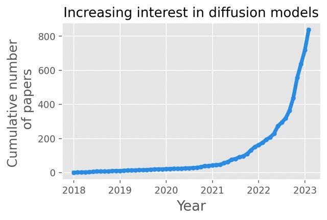
Caption: Number of papers on diffusion in recent years. Source: [2]
Being spoiled for choice is usually a good thing, but keeping up is quite problematic – before you fine-tune your favorite new model, there is another state-of-the-art solution waiting to be explored. Important choices not only refer to the abstract topic of architecture. After selecting your weapon of choice, another rabbit hole opens up: parametrization. Each of the models and methods comes with dozens of parameters for both training and generation, with an exponential number of combinations. Both inherent variance in output quality and the lack of fixed criteria of what constitutes good results make the search for perfect parameters truly challenging.
All of that can leave even the toughest deep-learning practitioner confused. But don’t worry! In this and future posts, we would like to explain our empirical and data-based approach to enable rational assessment and choices. These helped us navigate the complications and we hope that it will be beneficial for others as well. Let’s dive into it!
Let’s assume that we managed to choose our favorite model. More than that, we adapted it to our needs via fine-tuning. That’s great news! But how can we assess the quality of our adjustments? The visual inspection always comes first, but when done ad-hoc it’s by no means informative nor reproducible. We would like to have a solution that is as automatic as possible, as well as being reliable.
Several natural metrics immediately come to mind, one of which makes it possible to establish how similar the output of our model is to the object that we embedded in the model domain during fine-tuning. Another can inform the user about the aesthetic value of the image. So how can we actually measure those? We decided to use the human-like approach i.e. look at the input/output images and estimate the performance of the model using subjective criteria. The metrics described below were proposed and validated based on one specific type of object: faces.
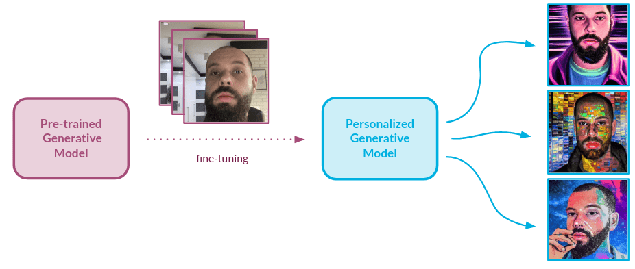
Caption: Personalized face generation process. Source: Authors
However, with small adjustments, the approach we describe below can be applied to any domain. Most importantly, the general methodology for the validation can be used for any generative setup.
Our goal is to gather insights into how well the model understands the images that were provided during the training, or in our case, fine-tuning. The similarity of object’s characteristics between real picture and the output is vital for a high-quality model. To make sure the model has acquired knowledge about the characteristics of new objects, there is a need for a validation setup that provides information about how similar the object is to the generated image when compared to the dataset used for fine-tuning.
Usually, we would like the model to generate our object in different setups, styles, and scenarios. A different textual input prompt means different colors and textures in the images. What we truly care about is how well our model conveys the characteristics of the object to an image.
To measure that, we use a two-stage solution – first, we crop out the object from pictures, as this is the only part we want to measure the similarity for. Next, we embed the images using an Inception-based [5] neural network. Let’s talk about those models and the validation scheme we used to make sure they are the right fit for our approach.
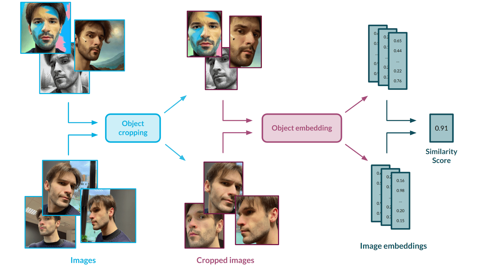
Caption: Similarity assessment flow. Source: Authors
We opted for the MTCNN [6] architecture which is specifically trained for the task of face cropping, but a similar architecture can be applied to any other type of object. This solution is based on several Convolutional Neural Networks that work in a cascade fashion to locate the face with some landmarks in an image.
The first network is called a Proposal Network – it parses the image and selects several bounding boxes that surround an object of interest: a face, in our case. It is the fastest of all three networks since its main job is to perform basic filtering and produce a number of candidate boxes. In the second step, the candidates are fed into a Refine Network, which further reduces the number of false candidates and refines the bounding box locations. The third and last network, the Output Network, performs the final adjustments and additionally provides information about facial landmarks. In this model, the location of 5 landmarks is predicted – the left and right eyes, the left and right corners of the mouth, and the nose.
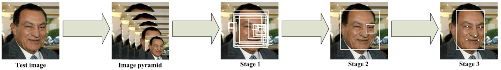
Caption: MTCNN architecture. Source: [7]
Needless to say, other tools can be applied with similar effects here, including architectures that are not designed to work with facial images.
Having extracted the faces, we opted for InceptionResnetV1 [8] as an encoder to allow for reliable comparison. This model can boil the input down to a numerical representation, which allows it to represent the abstract images in a pleasant, vector form. It was originally trained on the VGGFace2 [9] dataset containing 3.31 million images across over 9000 identities. In the case of other objects, other versions of the Inception-based network could be used.
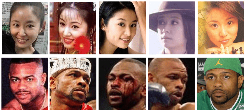
Caption: Sample images of Ruby Lin and Roy Jones Jr. from the VGGFace2 dataset. Source: [9]
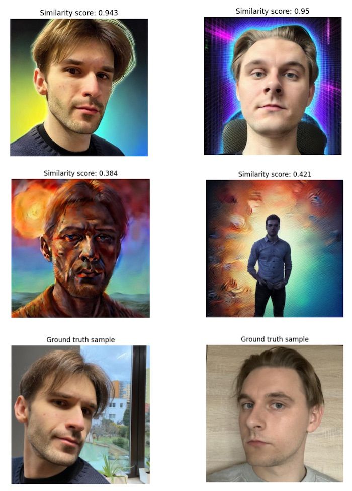
Caption: Examples of generated images with different similarity scores. Source: Authors
How does it work? InceptionResnetV1, trained beforehand on a significant number of different faces, can extract their features and encode their representations in a way that the similar faces are represented through vectors that lie close together in vector space.
Aesthetic measurement is a second important metric that helps to establish how powerful a model is. Image aesthetics is a pretty abstract concept, which is difficult to grasp and define even for a human. Strictly defining it with mathematical formulas could prove impossible; hence, we decided to model it using data. For that purpose, we used a publicly available dataset with subjective aesthetic assessments gathered from people. To best represent the images, we decided on the CLIP [10] model from OpenAI – the same architecture that is used in the Stable Diffusion [3] pipeline. CLIP works as a well-defined mapping between images and text – we covered it in a previous post in this series [1].
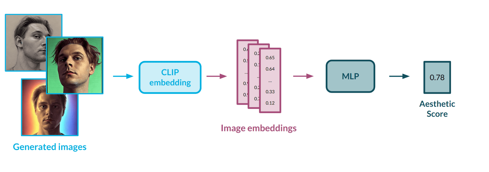
Caption: Aesthetic assessment flow. Source: Authors
Having a way to represent images in numerical form, there was a need to automate the process of evaluating the aesthetics of a given image. To do this, we used an AVA dataset [11] containing more than 250,000 images, along with assessments of their aesthetics by various people. Our goal was to train a multi-layer neural network in a regression setup to teach it the abstract correlation between face characteristics and aesthetic value. The model would rate each image on a scale from 0 (poor aesthetics) to 10 (great aesthetics). We applied data balancing methods to the input dataset to influence the rating distribution, as the first model’s outputs were highly condensed in the middle of the scale – the model had problems estimating extreme values, e.g., 1-2 or 9-10.

Caption: Examples of generated images with low and high aesthetic scores. Source: Authors
It is worth noting that the LAION dataset [12] on which Stable Diffusion was trained also has aesthetic evaluations. While it might have been easier to use that one, it could lead to unwanted data leakage, which is why we depended on an external dataset.
Enough talk! That was a comprehensive description of the metrics – it is time to see how they work. Let’s ask ourselves one of the many valid questions we might have when thinking about model fine-tuning – how many input images do I need to use?
The graph above should help you find the answer to that question. It is fully interactive, so feel free to explore it. We fine-tuned the Stable Diffusion v1.5 model on pictures of several people, and tested a different number of input images to see how it affects the training of the model. You can trace how different metrics behave during the evaluation every 300 steps and how it affects the images produced.
Visual inspection allowed us to notice that the presented metrics work well, scoring comparably to humans. However, we would not feel comfortable without validating those setups, so we decided to make sure we can rely on them to provide us with accurate information. We strongly recommend you visit Appendix A to see exactly how it was done!
In this post, we expressed how confusing it might be to successfully navigate the convoluted area of diffusion models, in both a theoretical and practical sense. To make matters simpler, we introduced two metrics that come in very handy when a reliable assessment of the models is needed. We proved that these models are well-balanced and suitable for our needs with comprehensive validation. In the next post of this series, we will expand on this approach, with lots of experiments and more metrics to check them. Stay tuned!
For validation purposes, we used images of 8 different people – 4 women and 4 men – to fine-tune 8 new v1.5 Stable Diffusion models. We used the same number of images to fine-tune the models for all of the subjects. After training, two evaluation datasets were created by generating 128 pictures with each model, using half of the images for similarity validation and the other half for aesthetic validation.
Five different people marked the aforementioned sets of pictures according to their subjective opinion. Each image received a label from 1 to 5 (Likert scale [13]) from each labeler, with one meaning very bad and five being very good. This type of labeling was done for both metrics separately. After that, we could calculate several statistics, such as each evaluator’s grade, which is essentially a mathematical formulation of how the given labeler assesses the images. For all of the proper definitions, please check out Appendix B of this post.
Every set was then divided into 5 cross-validation sets in a 4:1 ratio considering the labeler’s dimension – in each set, the labels from one labeler were included in the test set. Using our proposed evaluation as the function we want to optimize, we undertook model score mapping (bucket division) on a scale of 1 to 5 on the validation sets. We performed the bucketizing in a way that minimizes the distance between the model and human answers.
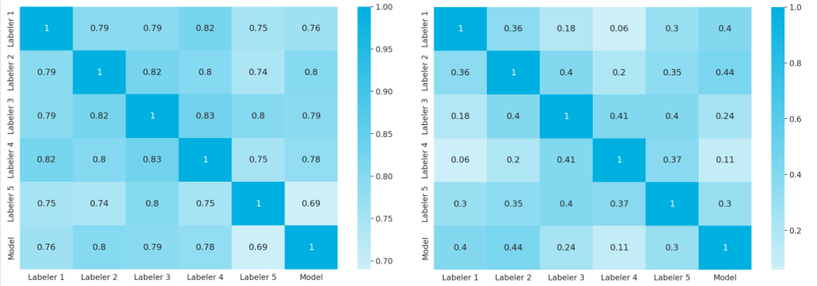
Caption: Spearman’s coefficient scores for labelers and models – similarity model evaluation on the left, and aesthetic model evaluation on the right. Source: Authors
Next, we tested the model score (similar to the test set labeler) and averaged it out over 5 test sets. We can observe that there is a highly positive correlation between human labels and the score predicted by the similarity model.
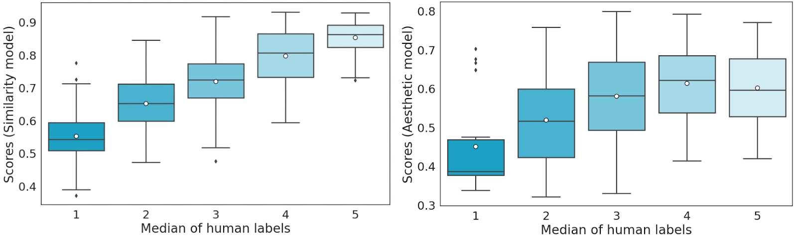
Caption: Comparison of human labeling and assessment model scores. Source: Authors
In the table below we present the results of cross-validation of the model. After optimization, the models perform in a human-like fashion – exactly what we aimed for!
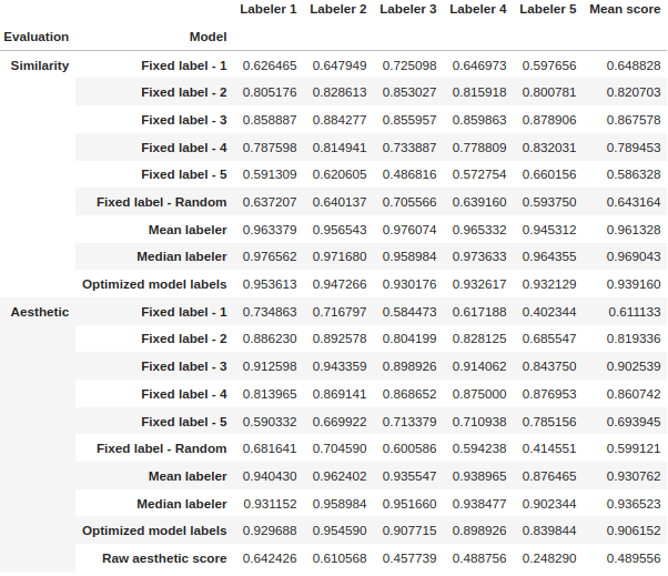
Caption: Table comparing results of different models. Source: Authors
Let’s denote \(E\) as the set of evaluators of a given set of images \(S\). We can formulate a discrete Likert scale evaluation as
$$
\begin{equation}
\forall e \in E \;\; \forall s \in S \quad e_d(s) \in L.
\end{equation}
$$
Each score is normalized so that the scores are within the \([0, 1]\) interval, which we can describe as a scoring function \(e\):
\begin{equation}
\forall e \in E \;\; \forall s \in S \quad e(s) \in [0,1].
\end{equation}
For each evaluator, we can define a mean evaluator score on the set of images \(S\) as
\begin{equation}
\forall e \in E \quad \bar{e}=\dfrac{\sum\limits_{s \in S} e(s)}{|S|}
\end{equation}
as well as the standard deviation of the evaluator score on the set of images S
\begin{equation}
\forall e \in E \quad \sigma(e)=\sqrt{\dfrac{\sum\limits_{s \in S}(e(s)-\bar{e})^{2}}{|S|}},
\end{equation}
where \(|S|\) denotes the cardinality of the set of images.
For a single image sample, we can define a sample score \(\bar{s}\) as
\begin{equation}
\forall s \in S \quad \bar{s}=\dfrac{\sum\limits_{e \in E} e(s)}{|E|}.
\end{equation}
Specifically for the single evaluator grading, we include a modification of the above score \(s\) established for each labeler. Let’s denote \(E_{e}\) as the set of evaluators without evaluator \(e(\forall e \in E \; E_{e} = E\setminus{e})\). We can define a sample score without the evaluator \(e\) as:
\begin{equation}
\forall e \in E \;\; \forall s \in S \quad \bar{s}_e=\dfrac{\sum\limits_{e \in E_e} e(s)}{\left|E_e\right|}.
\end{equation}
For a single evaluator \(e\) we can define his grade on the set of images \(S\), denoted as \(g(e)\), which is referred to as evaluator’s grade
\begin{equation}
\forall e \in E \quad g(e)=1-\frac{\sum\limits_{s \in S}\left|e(s)-\bar{s}_e\right|^k}{|S|},
\end{equation}
where \(k \in \mathbb{N}+\) is a grading parameter.

Large language models (LLMs) are yielding remarkable results for many NLP tasks, but training them is challenging due to the demand for a lot of GPU memory and extended training time. This is compounded by the fact that the size of many models exceeds what a single GPU can store. For instance, to fine-tune BLOOM-176B, one would require almost 3 TB of GPU memory (approximately 72 80GB A100 GPUs). In addition to the model weights, the cost of storing intermediate computation outputs (optimizer states and gradients) is typically even higher. To address these challenges, various parallelism paradigms have been developed, along with memory-saving techniques to enable the effective training of LLMs. In this article, we will describe these methods.
In data parallelism (DP), the entire dataset is divided into smaller subsets, and each subset is processed simultaneously on separate processing units. During the training process, each processing unit calculates the gradients for a subset of the data, and then these gradients are aggregated across all processing units to update the model’s parameters. This allows for the efficient processing of large amounts of data and can significantly reduce the time required for training deep learning models.

Figure 1: Illustration of data parallelism. Source: [11]
Since deep neural networks typically have multiple layers stacked on top of each other, the naive approach to model parallelism involves dividing a large model into smaller parts, with a few consecutive layers grouped together and assigned to a separate device, with the output of one stage serving as the input to the next stage. For instance, if a 4-layer MLP is being parallelized across 4 devices, each device would handle a different layer. The output of the first layer would be fed to the second layer and so on, until the last layer’s output is produced as the MLP’s output.
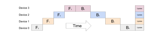
Figure 2: The naive model parallelism strategy is inefficient because the network works in a sequential manner and can only use one accelerator at a time. Source: [3]
To address the need for efficient pipeline parallelism, in 2019 researchers at Google introduced a new technique for parallelizing the training of deep neural networks across multiple GPUs – GPipe (Huang et al. 2019).
Unlike naive model parallelism, GPipe splits the layers in a way that maximizes parallelism while minimizing communication between GPUs. The key idea behind GPipe is to partition theincoming batch into smaller micro-batches, which are processed in a distributed manner on the available GPUs. The GPipe paper found that if there are at least four times as many microbatches as partitions, the bubble overhead is almost non-existent. Furthermore, the authors of the paper report that the Transformer model exhibits an almost linear speedup when the number of microbatches is strictly larger than the number of partitions.
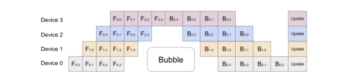
Figure 3: GPipe splits the input mini-batch into micro-batches, which can be processed by multiple accelerators at the same time. Source: [3]
In tensor parallelism, specific model weights, gradients and optimizer states are split across devices and each device is responsible for processing a different portion of the parameters.
In contrast to pipeline parallelism, which splits the model layer by layer, tensor parallelism splits individual weights. In this section we will describe the technique for parallelizing a Transformer model with tensor parallelism using an approach that was proposed in the Megatron-LM paper (Shoeybi et al. 2020).
A Transformer layer consists of a self-attention block followed by a two-layer perceptron. First, we will explain the MLP block.
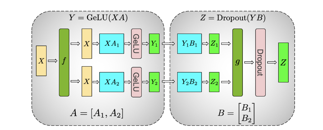
Figure 4: Illustration of tensor parallelism for the MLP block. Source: [5]
$$
[Y_1, Y_2] = [GeLU(XA_1), GeLU(XA_2)].
$$
In this way, a synchronization point can be skipped. The second GEMM operation is performed such that the weight matrix \(B\) is split along its rows and input \(Y\) along its columns:
$$
Y = [Y_1, Y_2], B = [B_1, B_2]^T,
$$
resulting in \(Z = Dropout(YB) = Dropout(Y_1B_1 + Y_2B_2)\).
We will now move on to the explanation of the self-attention block.
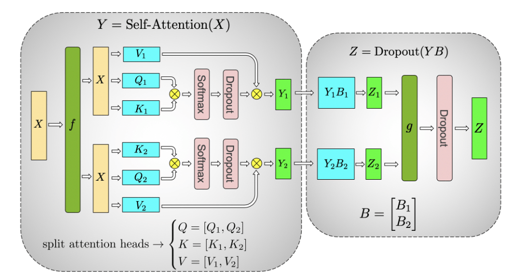
Figure 5: Illustration of tensor parallelism for the self-attention block. Source: [5]
$$
Attention(Q, K, V) = softmax \big( \frac{QK^T}{\sqrt{d_k}} \big) V.
$$
To measure the scalability of their implementation, the authors of the MegatronLM paper considered GPT-2 models with \(1.2, 2.5, 4.2\) and \(8.3\) billion parameters. They evaluated both tensor parallelism and a combination of tensor parallelism with 64D data parallelism which demonstrated up to 76% scaling efficiency using 512 GPUs. Mixed Precision Training and Activation Checkpointing techniques were also used – we elaborate more in the following paragraphs.
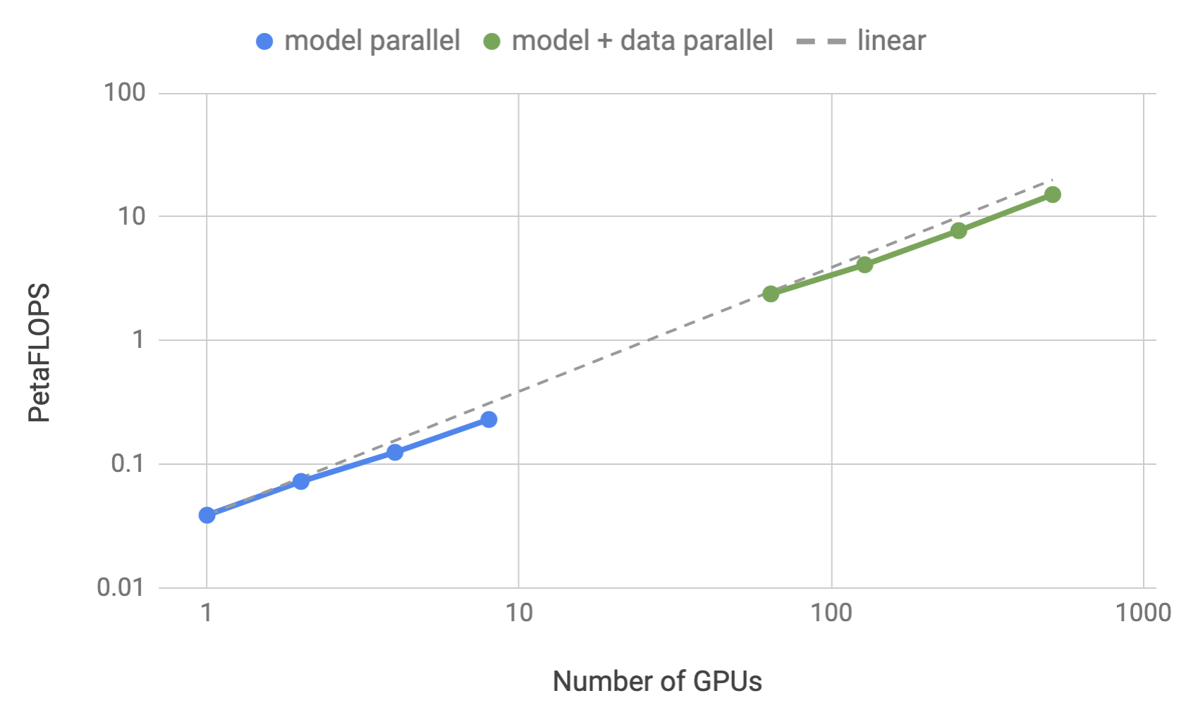
Figure 6: Training efficiency for tensor parallelism and a combination of tensor parallelism with data parallelism as a function of the number of GPUs. Source: [5]
Another method to parallelize computation across multiple devices is Sequence Parallelism (Li et al. 2021), a technique for training Transformer models on very long sequences by breaking them up into smaller chunks and processing each chunk in parallel across multiple GPUs.
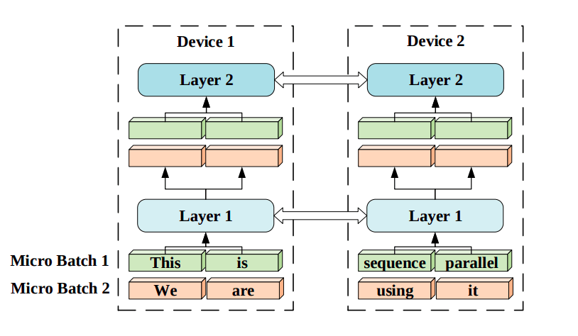
Figure 7: Sequence parallelism illustration. Input sequences are divided into smaller pieces and distributed to corresponding devices. Each device has the same trainable parameters but different sub-sequence input chunks. Source: [7]
We begin by establishing some notations which we adopt from the original paper. We assume that the embeddings on the n-th device correspond to the n-th chunk of the input sequence and are denoted as \(K^n\) (key), \(Q^n\) (query), and \(V^n \) (value). Additionaly, we set the number of available GPUs to \(N\).
The goal of the first stage of RSA is to compute \(Attention(Q^n, K, V)\) which is the self-attention layer output on the n-th device. To achieve this, the key embeddings are shared among the devices and used to calculate attention scores \(QK^T\) in a circular manner. This requires \(N-1\) rounds of communication. As a result, all attention scores \(S^1, S^2, \dots, S^N\) are stored on the proper devices.
In the second stage of RSA, the self-attention layer outputs \(O^1, O^2, \dots, O^N\) are calculated. For this purpose, all value embeddings are transmitted in a similar way as the key embeddings in the previous stage.
The fundamental concept behind the Mixture-of-Experts method (MoE, Shazeer et al. 2017) is ensemble learning. To go into more detail, the MoE layer consists of a set of \(n\) feed-forward expert networks \(E_1, E_2, \dots, E_n\) (which can be distributed across GPUs) and the gating network \(G\) whose output is a sparse \(n\) -dimensional vector. The output \(y\) of the MoE layer for a given input \(x\) is
$$
y = \sum\limits^{n}_{i=1} G(x)_i E_i(x),
$$
where \(G(x)\) denotes the output of the gating network and \(E_i(x)\) – the output of the \(i\)-th expert network. It is easy to observe that wherever \(G(x)_i = 0\) there is no need to evaluate \(E_i\) on \(x\).
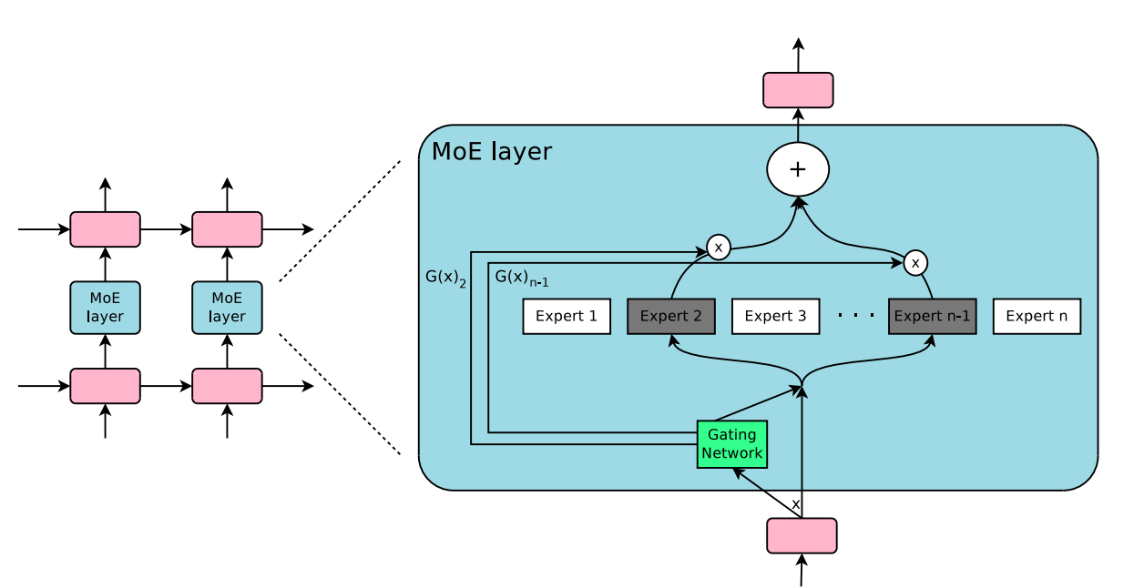
Figure 8: Illustration of a mixture-of-experts (MoE) layer where the gating network activates only two of the experts. Source: [8]
$$
G(x) = Softmax(KeepTopK(H(x), k))
$$
$$
H(x)_i = (x \cdot W_g)_i + \epsilon \cdot softplus((x \cdot W_{noise})_i), \epsilon \sim N(0, 1),
$$
$$
KeepTopK(v, k)_i = v_i \mbox{ if } v_i \mbox{ is in the top } k \mbox{ elements of } v, -\infty \mbox{ otherwise }.
$$
Suppose we partition a neural network into k partitions. In Activation Checkpointing (Chen et al. 2016), only the activations at the boundaries of each partition are saved and shared between workers during training. The intermediate activations of the neural network are recomputed on-the-fly during the backward pass of the training process rather than storing them in memory during the forward pass.
Two common floating-point formats used in Deep Learning applications are the single-precision floating-point format (FP32) and the half-precision floating-point format (FP16). The half-precision data type uses 16 bits to represent a floating-point number, with 1 bit for the sign, 5 bits for the exponent, and 10 bits for the significand. On the other hand, FP32 uses 32 bits, with 1 bit for the sign, 8 bits for the exponent, and 23 bits for the significand.
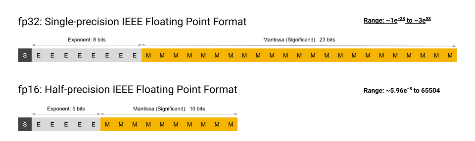
Figure 9: FP16 and FP32 formats. Source: [16]
which can be beneficial in applications where speed and reduced memory usage are more important than accuracy, such as in Deep Learning models that require a large number of calculations. However, FP16 is less precise than FP32, which means that it can result in rounding errors when performing calculations.
The concept of Mixed Precision Training (Narang & Micikevicius et al. 2018) bridges the gap between reducing memory usage during training and maintaining good accuracy.
Mixed Precision Training involves utilizing FP16 to store weights, activations, and gradients. However, to maintain accuracy similar to that of FP32 networks, an FP32 version of the weights (the master weights) is also kept and modified using the weight gradient during the optimizer step. In each iteration, a copy of the master weights in FP16 is utilized in both the forward and backward passes, which reduces storage and bandwidth requirements by half compared to FP32 training.
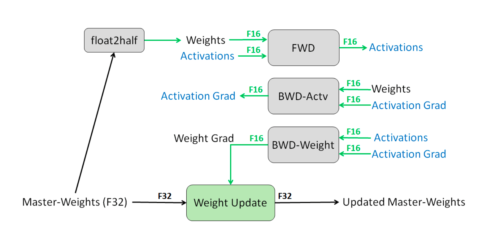
Figure 10: Mixed precision training process. Source: [9]
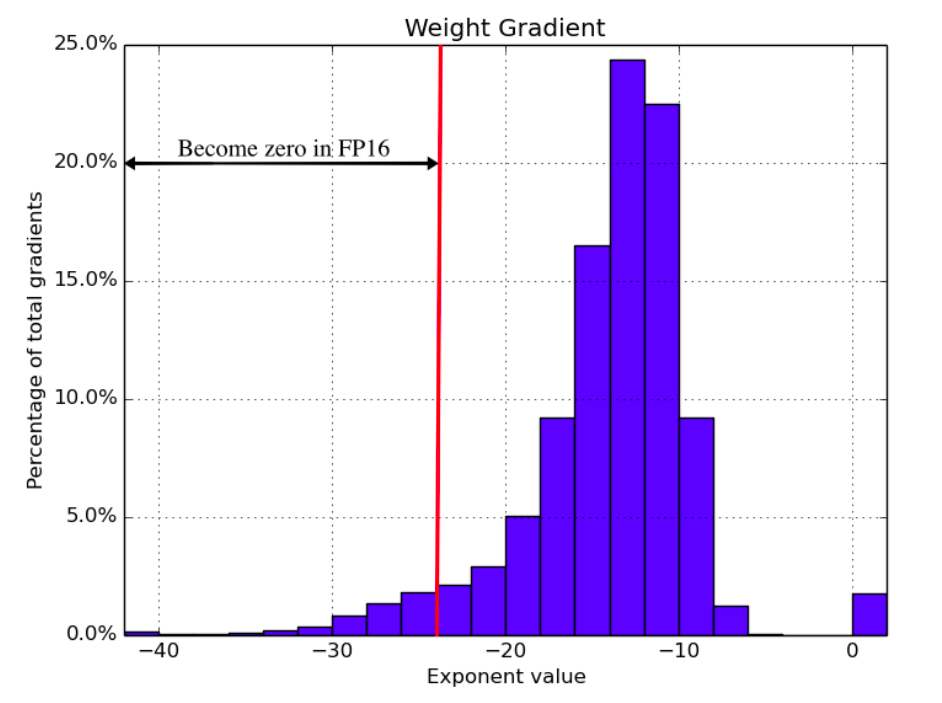
Figure 11: The distribution of weight gradient exponents when training a speech recognition model with FP32 weights. Source: [9]
The authors of “Mixed Precision Training” also provide experimental results showing the effectiveness of the technique on image classification and language translation tasks. In both cases, Mixed Precision Training matched the FP32 results.
Optimizers use a lot of memory. For example, while using the Adam optimizer, we need to save four times the memory of model weights, as it stores momentums and variances which are as big as the gradients and model parameters (Weng 2021).
All parallelism techniques described in the previous sections store all the model parameters required for the entire training process, even though not all model states are needed during training. To address these drawbacks of training parallelism while retaining the benefits, Microsoft researchers developed a new memory optimization approach called Zero Redundancy Optimizer (ZeRO, Rajbhandari et al. 2019).
ZeRO aims to train very large models efficiently by eliminating redundant memory usage, resulting in better training speed. It eliminates memory redundancies in Data Parallel processes by dividing the model states across the devices instead of duplicating them.
ZeRO has three optimization stages:

Figure 12: Three optimization stages of ZeRO compared with the data parallelism baseline. Source: [13]
Making Transformers understand longer inputs is difficult because their multi-head attention layer needs a substantial amount of memory and time to process the input, and this requirement grows quadratically with the length of the sequence. When training Transformers on long sequences with parallelism techniques described in previous sections, the batch size can become extremely small. This is the scenario which the FlashAttention method (Dao et al. 2022) improves.
To optimize for long sequences for each attention head, FlashAttention splits the input \(Q, K, V\) into blocks and loads these blocks from GPU HBM (which is the main memory) into SRAM (which is its fast cache). Then, it computes attention with respect to that block and writes back the output to HBM.
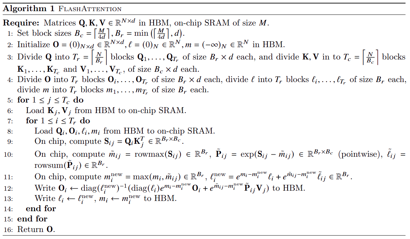
Figure 13: FlashAttention algorithm. Source: [14]
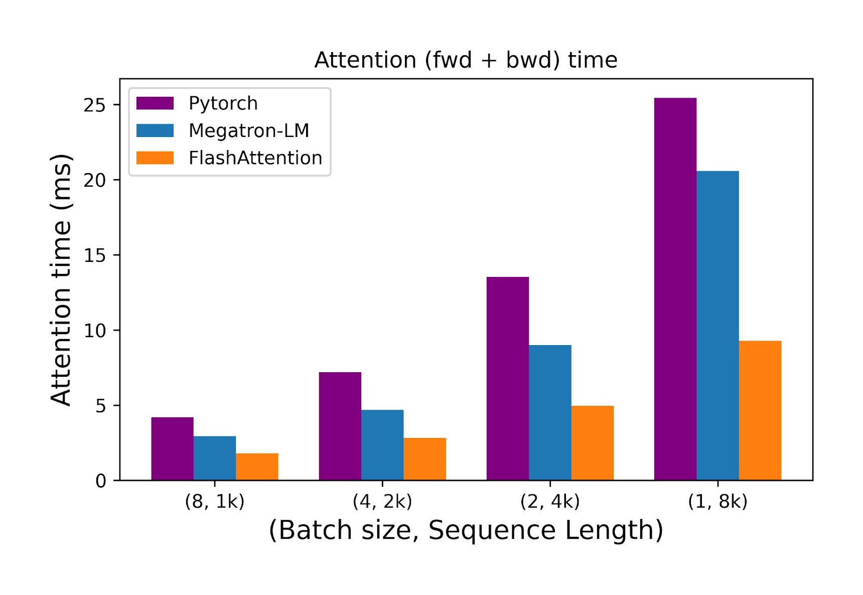
Figure 14: Comparison of the time taken by the forward and backward passes of the attention layer as the sequence length increases while the batch size decreases. Source: [15]
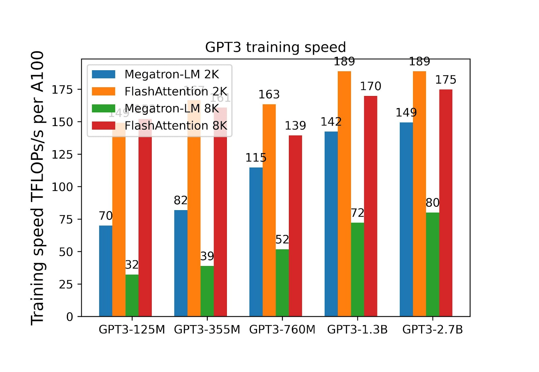
Figure 15: Training efficiency as a function of the model size. Source: [15]
In the article, various memory optimization techniques for training large language models were discussed. We explained different parallelism paradigms: Data Parallelism, Naive Model Parallelism, Pipeline Parallelism, Tensor Parallelism and Sequence Parallelism. In addition, some pros and cons of these approaches were presented. We then moved on to other memory optimization methods: Mixture-of-Experts, Mixed Precision Training and ZeRO (Zero Redundancy Optimizer). While explaining Mixed Precision Training, we also went through the Loss Scaling technique. Finally, we introduced FlashAttention – an algorithm dedicated to memory reduction for the attention layer.
To sum up, we’ve presented several methods that it’s important to be familiar with when training large language models, as these methods can help improve the efficiency, scalability, and cost-effectiveness of the training, as well as optimizing resource utilization.
Are you ready to explore the potential of large language models like GPT? Join our GPT and other LLMs Discovery Workshop to start your AI journey today.

It is widely known that computer vision models require large amounts of data to perform well. The reason for this is the complexity of these tasks, which usually involve the recognition of many different features, such as shapes, textures, and colors. Therefore, to train state-of-the-art, advanced models, it is necessary to use vast datasets like, for example, ImageNet, containing 14 million images.
Unfortunately, in many business cases we are left with a small amount of data. Small datasets may be due to the high cost of data collection, privacy concerns, or the limited availability of data. This causes various problems such as underrepresentation of the rarest classes, being prone to overfitting and the limitations of the machine learning algorithms or deep learning models that can be used.
When working with limited data, it can be difficult to train a model that is accurate and generalizes well to new examples. There are several approaches to overcoming the issue of insufficient data, one of which is supplementing the available dataset with new images, which is discussed in this article.
Diffusion models are a class of generative models that have become increasingly popular in recent years due to their ability to generate high-quality images. At a high level, diffusion models work by firstly adding a certain amount of random noise to the images from the training set. Then the reverse process happens, that is, during training the model learns to remove the noise to reconstruct the image. The advantage of this approach is that it allows the model to generate high-quality samples that are indistinguishable from real data, even with a small number of training examples. This is particularly useful in situations such as in medical imaging, where obtaining high-quality images is expensive and time-consuming. Popular diffusion models include Open AI’s Dall-E 2, Google’s Imagen, and Stability AI’s Stable Diffusion.
You can read more about the recent rise of diffusion-based models in our recent post.
In recent years, there has been growing interest in the application of diffusion-based models in creating new images based on those which already exist. Many architectures modify the baseline to achieve the best quality of output. Below we discuss a few of them, to give you an overview of what can be accomplished.
One of the fields where there is a need to complement datasets is medical imaging. The use of real patient data is encumbered with privacy and ethical concerns. What is more, there is a lack of process standardization when it comes to sharing sensitive data, even between hospitals and other medical research facilities. To overcome the barrier of privacy issues and a lack of available medical data, Medfusion architecture was proposed by Muller-Franzes et al. in [1].
In the past, it was common to use generative adversarial models (GANs) to generate data based on existing training data. However, it has been proven that GANs suffer from unstable training behavior, among other things [2].
In [1] the authors present a novel approach based on Stable Diffusion [3]. The model consists of two parts: an autoencoder and a Denoising Diffusion Implicit Model (DDIM). The autoencoder compresses the image space into a latent space. During training, the latent space is decoded back to the image space. Then they use a pre-trained autoencoder to get the image to the latent space which is then diffused into Gaussian noise. A UNet model is used to denoise the latent space, and samples are generated with the DDIM. During their research they first investigated whether the autoencoder was sufficient to encode images into a compressed space and decode them back without losing medically relevant details. Then they studied whether the Stable Diffusion Model’s autoencoder, pre-trained on natural images, could be used for medical images without further training. The results showed that the Medfusion model was effective in compressing and generating images while retaining medically relevant details, and the Stable Diffusion Model’s pre-trained autoencoder could be used for medical images without the loss of any relevant details, and could outperform GANs in terms of the quality of output images. The study highlights the potential of the Medfusion model for medical image compression and generation, which could have significant implications for healthcare providers and researchers.
They explored three domains of medical data: ophthalmologic data (fundoscopic images), radiological data (chest x-rays) and histological data (whole slide images of stained tissue).
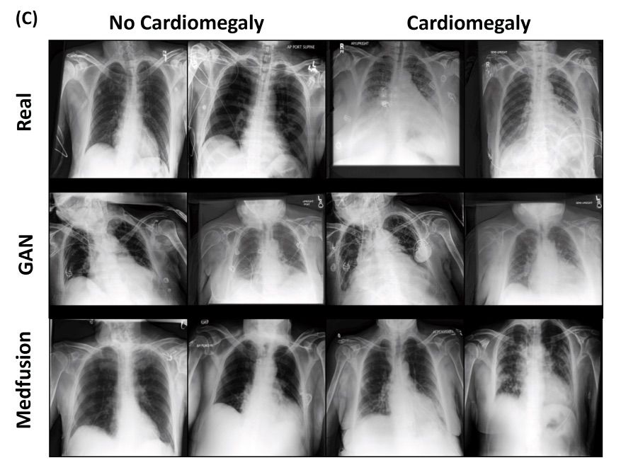
Figure 1. Qualitative image generation comparisons. Image from [1].
While working with diffusion models, one can encounter the problem that the output changes even in terms of the parts of the picture that we would like to stay the same. In the case of generating new images to supplement the existing dataset, we would prefer, e.g., the semantic masks or the edges (possibly obtained by Canny or Hugh lines detector) that we already have to still apply to the newly created image.
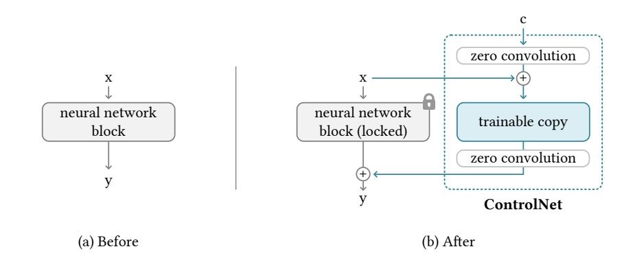
Figure 2. ControlNet architecture overview. Image from [4].
The authors trained several ControlNets with various datasets of different conditions, such as Canny edges, Hough lines, user scribbles, human key points, segmentation maps, shape normals, and depths. The results showed that ControlNet was effective in controlling large image diffusion models to learn task-specific input conditions.

Figure 3. Control Stable Diffusion with Canny edge map. Image from [4].
Standard data augmentation techniques are image transformations such as flips, rotations or changes in color. Unfortunately, they do not allow more sophisticated changes in the appearance of the object. Suppose we would like to have a model detect and recognize a plastic bottle in the wild, e.g., while creating a waste detector – it would be very helpful to be able to vary the appearance of the bottle in terms of the label or the color of the bottle, etc. Unfortunately this is not possible with classical data augmentation. The DA-Fusion [5] method, based on text-to-image diffusion models, was proposed to address this issue.
The authors utilize pre-trained diffusion models to generate high-quality augmentations for images, even those with visual concepts not previously known to the base model. In the text-encoder, new tokens were used to adapt the diffusion model to new domains. In order to do so, Textural Inversion [6] was applied – a technique for capturing novel concepts in the embedding space of a text encoder.
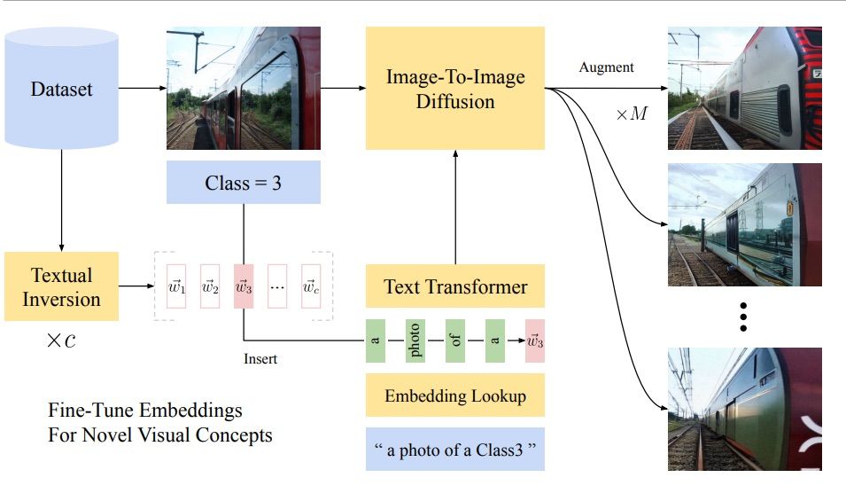
Figure 4. System architecture for DA-Fusion. Image from [6].
At deepsense.ai we strongly believe that data is crucial to the performance of machine learning models. Therefore, we are constantly searching for new approaches to make the most of the data that we have available. Recently, we have been exploring the use of generative models as well as novel diffusion models and variations thereof.
Stay tuned for our next post to find out more about our approach to applying these methods to synthesizing datasets from different domains (i.e. medical images, street view) for classification and segmentation tasks.

The AI revolution continues, and there is no indication of it nearing the finish line. The last year has brought astonishing developments in two critical areas of generative modeling: large language models and diffusion models. To learn more about the former, check out other posts [1] by deepsense.ai. This series is devoted to sharing our practical know-how of diffusion models.
Application of the family of models using a mechanism called “diffusion” in various generative setups remains one of the hottest topics in machine learning. Diffusion-based models have proven their ability to yield results surpassing all other well-known counterparts used in this domain beforehand, such as Generative Adversarial Networks (GANs) or Variational Autoencoders (VAEs). Sohl-Dickstein et al.’s [2] publication in 2015 brought a breath of fresh air to the generative model scene. For a few years, the concept was gradually improved upon, and just last year there were numerous state-of-the-art publications in the domain of image-to-image, text-to-audio, and time series forecasting, just to name a few. The number of applications is growing by the day, although the text-to-image domain remains the most popular so far – we are focusing solely on it in this series as well. There are many practical questions one may have when trying to use these methods, such as:
These and similar questions have both beginners and advanced practitioners struggling. While the Internet is full of math-heavy theories and opinionated claims, there are not many well-researched answers to these questions available. Over the next few posts, we intend to present a practical and empirical answer to them.
The series will contain the results of multiple experiments using various models and metrics. Based on these, we will present insights which are relevant to the specific practical dilemmas and challenges, and allow you to draw your own conclusions by facilitating a graphical, interactive exploration of these results.
First, however, this post will lay the groundwork for this with just enough theory to make the following ones understandable. We will introduce the relevant tools and concepts to be referenced in later posts, and we strongly recommend familiarizing yourself with them. More specifically, we will introduce Stable Diffusion [3] (one of the loudest models published last year) and several tools used to finetune it, including DreamBooth [4], LoRA [5], and Textual Inversion [6].
While DALL·E [7] and DALL·E 2 [8] were responsible for drawing large-scale attention to generative image models, Stable Diffusion [3] was the model that unleashed a true revolution. Since its open-sourcing in August 2022, anyone could modify, expand, tweak, or simply use it on their GPU or in a collab [9] for free. Follow-up technologies appeared, including training methods like DreamBooth [4], allowing people to see themselves (or anyone else) as a character in their generative art. The landscape of generative models (and possibly of art itself [10]) changed forever.
While ‘Stable Diffusion’ sounds catchy, for someone starting their adventure in the generative realm, the term ‘diffusion’ may be confusing. Within the context of deep learning, diffusion refers to one of the processes used by these methods to generate images based on the training data. That is, admittedly, a bit vague. How exactly do diffusion models differ from GANs, VAEs, or other models used in image modeling?
There are numerous novelties proposed. Essentially, various generative architectures are composed of two processes that are complementary to each other. GANs architectures utilize a generator and discriminator, while VAEs use an encoder and decoder setup. For diffusion-based models, it is no different, as we can formulate the model with two processes – diffusion (noising) and denoising [11].
Diffusion – also referred to as the forward diffusion process – is meant to sequentially destroy the image by slowly blurring the picture so that its main characteristics are no longer observable. One of the relatively new ideas for this family of models is that the formulation of this forward process is fixed. That is a large difference when compared to, e.g., VAEs, where both main components of the architecture are fully trainable. In the case of diffusion, the encoder’s job is overtaken by a mathematical process – the neural network approach is redundant.
The main goal of the entire architecture is to teach the model to reverse that process; to create something meaningful – an image – from a complete noise. This denoising process is performed by a neural network, and arguably this is the place where most of the heavy lifting is done. During the training, the network is presented with a diffused image and is taught to predict the noise added to it. When the predicted noise is subtracted from the input, a person/object/scene starts to emerge in the picture. As usual, the network is trained on millions of images and the feedback about its performance is constantly provided via loss function and backpropagation. The whole process allows the network to gather information about the characteristics of the pictures from the same class. We don’t tell the network explicitly how to reverse the diffusion process, since the generative power comes from the interpolation of the knowledge that the model gains during the training. Truth is, we wouldn’t even be able to do that, since it would require the model to have virtually infinite capacity (more about this in detail in [12]).
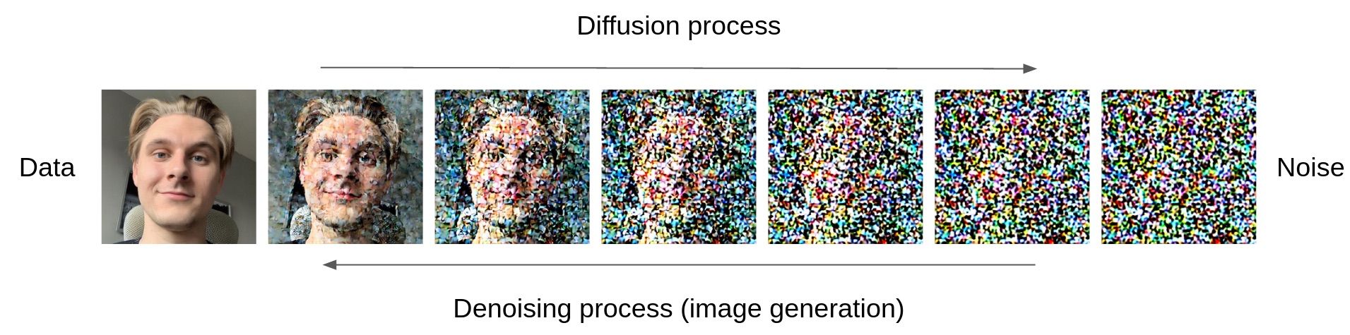
Visualization of the forward and reverse diffusion processes. Source: Authors’ own elaboration
That’s a very brief summary of the basics of the construction of diffusion models. We already have a detailed blog post [12] that focuses on the mathematical aspects. We covered DALL·E 2 [8] and Imagen [13] in detail there – we strongly recommend checking it out, as it should shed a great deal of light on the intricacies of diffusion in deep learning. In this section, we will give a general overview of the key terms and components of Stable Diffusion.
![Stable Diffusion architecture, source: [3]](https://deepsense.ai/wp-content/uploads/2023/03/Stable-Diffusion-architecture.jpeg)
Stable Diffusion architecture. Source: [3]
Below we will explain each of these in a bit more detail.
Diffusion models can work on their own, generating images based on the knowledge gained through the training process. Usually, we would like to be able to guide the generation process using text, so the model produces exactly what we want. This information is passed into the model in the form of a generation prompt. So how does the model understand the text?
When it comes to text-to-image generation, we can have the best of the generative and natural language processing worlds and successfully apply the solutions from one domain to the other. The area of Language Models has gained momentum rapidly in recent years. An increasing number of solutions allow for efficient embedding of the text in the abstract space, which later allows for efficient processing of the text in hand.
The idea of a text encoder is quite simple – we wish to take the textual input and represent it efficiently in a space that would allow the model to generate an image based on the prompt. That process is called text guidance – each time the diffusion model goes one step further in the image generation process, it is reminded of what the image was supposed to present. Currently, the choice of the model that transfers the text into a latent space seems paramount for accurate and high-quality generation. Many of the current state-of-the-art solutions utilize different architectures for text embedding. For instance, Imagen [13] architecture uses the T5-XXL [14], while Stable Diffusion uses the CLIP ViT-L/14 model [15] to get the job done.

CLIP model. Source: Authors’ own elaboration
CLIP [16] was trained with millions of (text, image) pairs and can accurately map the text to the image and vice versa. This makes it a very natural choice for the embedder, and it has already been proven to perform well, e.g., in DALL·E. The model itself is pre-trained and fixed in the Stable Diffusion, although there are ways to interfere with the embeddings – we will talk about those later in this post.
The heart of the solution – this part of the architecture takes the embedded text and noised latent and tries to reverse the diffusion process in a way that would produce an image as similar to the input prompt as possible. For anyone that follows neural network evolution, the way this is done may not be a great surprise. The weapon of choice is U-Net architecture, which was already used for lots of diffusion architectures before Stable Diffusion.
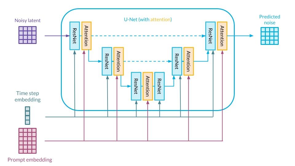
Overview of U-Net architecture. Source: Authors’ own elaboration
The denoising process happens step-by-step – each ResNet block receives the information about the denoising step and the text embedding is processed by the attention mechanism. A neural network aims to predict the noise that was added to the image during a forward pass of diffusion – that’s why the information about the step is important. During inference, the network tries to produce an image from a randomly sampled latent. The authors opted for the already well-established solution incorporating classifier-free guidance [17] to make sure that the image output is as close to the input text as possible.
The diffusion process itself is not very lightweight. Multiplying the height and width of the image, the number of color channels, and the number of noising steps in the process already leads to numerically heavy calculations. The authors of Stable Diffusion decided to address that by transferring the main part of the diffusion process into the latent space. Essentially the idea is to perform denoising not on the actual image in pixel dimensions, but rather to do it on a latent representation of the image, which is compressed to yield fewer dimensions. Historically there were already a few ways of performing this type of compression – the authors opted for an already well-known autoencoder approach.
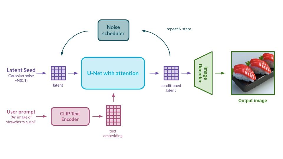
Example of the Stable Diffusion inference process. Source: Authors’ own elaboration
During the training, the input image is processed by the encoder and represented as latent several times smaller than the original e.g. 3x512x512 image is represented as a 6x64x64 matrix. It means that, in the architecture, all models work with a compressed representation of inputs that retains only the most valuable information. After the reverse diffusion process happens in U-Net, the tensor with all the necessary information for image generation is translated into the actual picture by the decoder.
To sum up, the flow seems easy enough – we type the text, and the encoder translates the text into a concise embedded form. The main model reverses the diffusion process of random noise in a step-by-step fashion, at the same time conditionally guiding the generation using the text. The last step is to take the model output and generate an image – that is the image decoder’s job. Our goal was to explain the interior of this architecture as simply as possible, but it needs to be underlined that actual model usage and navigating through the different parameters and settings is far more difficult! Worry not, as we will be helping with that as well.
November 2022 brought another iteration of the Stable Diffusion architecture – Stable Diffusion 2.0 [18]. Two weeks later, in December, Stability AI published the most recent stable version of the flag model to date – version 2.1 [19]. Just like its predecessor, it is available in the form of a demo [20]. There were a couple of major tweaks compared to the 1.5 version.
The new text encoder and dataset choice seem to be the largest of the changes. This time a newer generation OpenCLIP-ViT/H [21] model was trained to handle the task of text embedding. Just like its predecessor, CLIP ViT-L/14, its weights are open-sourced. The dataset used for the OpenCLIP training is open and includes several changes that drastically altered the way that model works with the prompts. An additional NSFW filter was included to filter out the images that could lead to misuse across the internet, mostly related to child abuse and pornography. Also, there is a noticeably smaller collection of celebrities and artistic images.
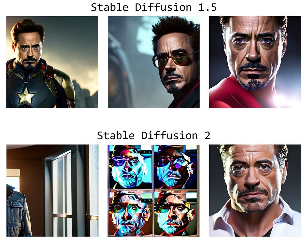
Comparison of generation for the prompt: “a studio photograph of Robert Downey Jr., cinematic lighting, hyperdetailed, 8 k realistic, global illumination, radiant light, frostbite 3 engine, cryengine, trending on artstation, digital art” for SDv1.5 and SDv2.0. Source: [22]
Additionally, negative prompting seems to be more important for accurate generation in the newer versions of Stable Diffusion. Negative prompts are appended to the regular generation prompt and should retain the information of what should not be seen on the generated picture. It was highly optional for the first version of the architecture, but it seems to be a must in the 2.0 and 2.1 versions in order to get high-quality results.
![Example of the importance of negative prompting in the 2.1 version. The pictures on both the left and right were generated with the same prompt, but there was an additional negative prompt added on the right to reduce the greenery in the image. Source: [19]](https://deepsense.ai/wp-content/uploads/2023/03/Example-of-the-importance-of-negative-prompting-in-the-2.1-version.jpeg)
Example of the importance of negative prompting in the 2.1 version. The pictures on both the left and right were generated with the same prompt, but there was an additional negative prompt added on the right to reduce the greenery in the image. Source: [19]
Although generative models offer endless possibilities, their domain knowledge can be limited. Often, the generation process relies on interpolating between images seen during training. While general pre-trained models are versatile, specific use cases may require additional training of the model. Since the release of Stable Diffusion as open-source software, several techniques have emerged to extend the knowledge of pre-trained models, collectively known as fine-tuning.
Several methods have been developed to generate specific objects, styles, or compositions with minimal data requirements. These techniques have pushed the boundaries of generative art even further. In the following chapters, we describe some established fine-tuning methods, some of which we used in our experiments.
This is one of the most popular methods, designed mainly to extend the model’s knowledge to include specific objects, but it is also possible to introduce styles (e.g. to incorporate a new artist). It works great for placing the face of a particular person in the model’s domain and more. It was also this method that we used for our internal Christmas card generator project – feel free to check it out [23].
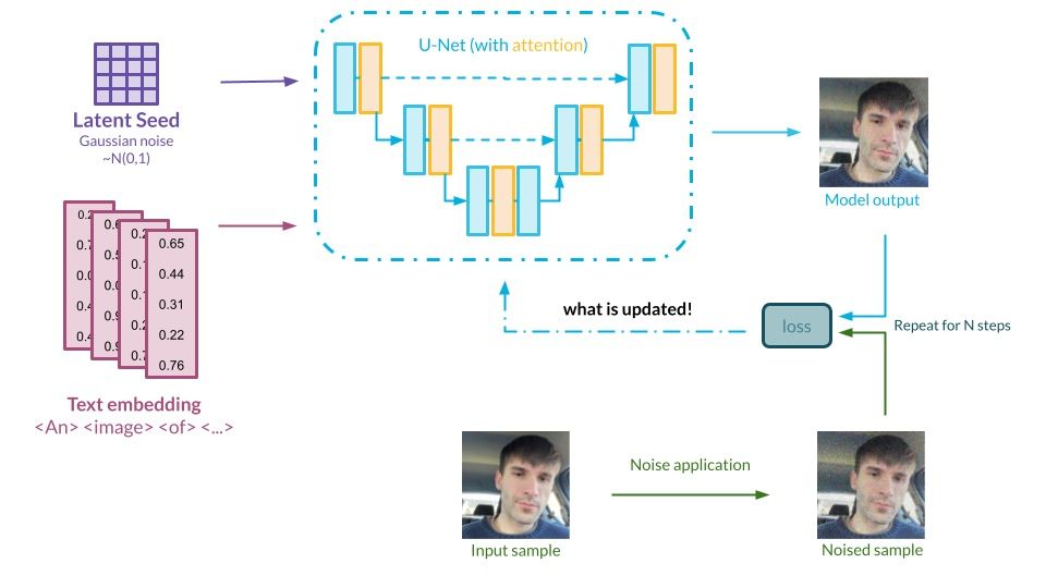
Graph presenting the DreamBooth method. Source: Authors’ own elaboration
When it comes to the technicalities, DreamBooth [4] is quite close to the traditional definition of fine-tuning.
In its basic form, it relies on freezing all weights of the architecture except for the U-Net model, which runs the denoising process. Additional training of the model is based on iteratively showing the network sample images of, e.g., the object of interest, along with a prompt containing a new, unique identifier to symbolize it, e.g., “A photo of a <identifier> dog”. The idea is to embed the knowledge about an object within the model weights and force it into the embedding layer. In the publication [4] the authors present a method for the rare-token selection to link with the identifier. The importance of choosing sparse tokens in this operation is not to be neglected – the model might lose some important information in the process.
Additionally, to combat overfitting and language drift, some regularization images with similar prompts are also shown during fine-tuning to ensure that the network does not forget the original meaning of the remaining tokens – this idea is called prior-preservation loss.
It is worth mentioning that DreamBooth implementation provided by Hugging Face [24] allows you to unfreeze the weight of the text encoder as well, which can further improve the results. On the other hand, it requires so much computing power that only a small percentage of users can launch these tools on their local machines. DreamBooth itself reigns supreme in terms of popularity among all methods listed in this post, but it comes with a price – it is the most computationally expensive. Even with the most basic setup, including numerous memory-efficient optimizations, this way of fine-tuning needs a GPU with 12GB of VRAM to perform training without major complications.
As of today, there are already hundreds of different concepts in the concepts library setup on Hugging Face – we strongly recommend checking them out [25].
LoRA [5] stands for Low-Rank Adaptation. It is not a diffusion-specific concept, as it was published in 2021 and targeted the problem of fine-tuning large language models such as GPT-3 [26]. These models, with millions of parameters, require a lot of storage, and altering the whole architecture each time there can be computationally expensive. Generally speaking, models are defined by parameters, which are stored in matrices. As the dimensions of the model increase, these matrices can grow very rapidly, which makes them heavy.
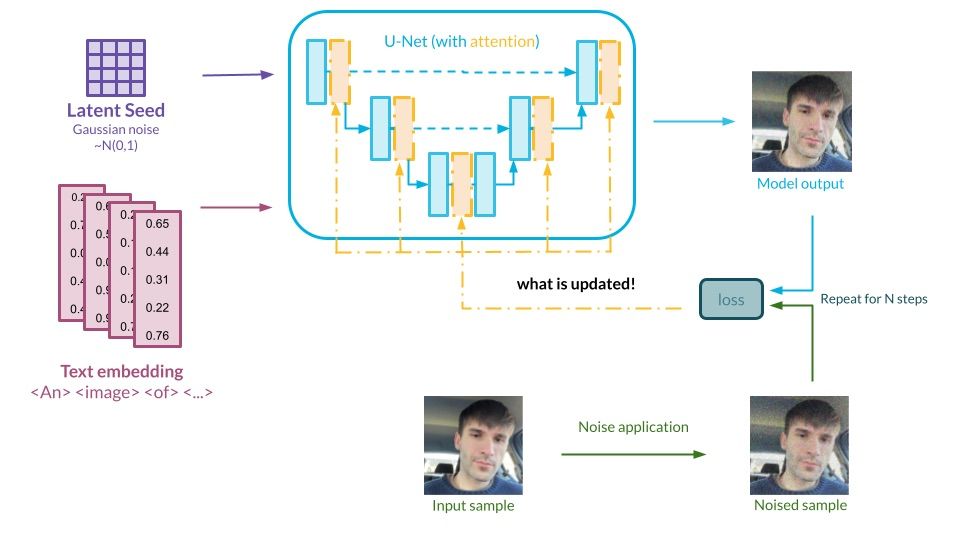
Graph presenting the LoRA method. Source: Authors’ own elaboration
In a nutshell, LoRA is a technique used to reduce the number of parameters that need to be tweaked to fine-tune the model. Instead of working with the whole matrices of parameters, these matrices are converted into a lower rank decomposition, which makes their size magnitudes smaller. On top of that, this technique does not need to be applied everywhere in the model. In the context of diffusion architectures – such as Stable Diffusion – the attention layers in the UNet network are specifically targeted, as they directly link the textual semantics with the generative ability of the model.
This approach yields several advantages:
Another powerful yet simple technique that can be used for adding new concepts to the model is called textual inversion [6]. It works by directly interfering with the text embedding layer of the architecture. The idea is similar to that of DreamBooth – we wish to give the model some information about a certain concept, potentially a new object or style, while maintaining the existing information.
![Inverting a visual idea of a specific cat into a <S∗> token. Source: [6]](https://deepsense.ai/wp-content/uploads/2023/03/Inverting-a-visual-idea-of-a-specific-cat-into-a-token.jpeg)
Inverting a visual idea of a specific cat into a <S∗> token. Source: [6]
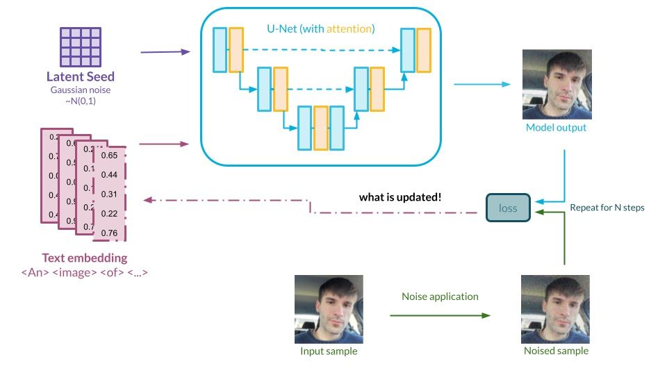
Graph presenting the textual inversion method. Source: Authors’ own elaboration
Hugging face offers a space [27] that showcases different new concepts that have been introduced into the embedding space of Stable Diffusion, such as <midjourney-style> or <nebula>.
The use of different training techniques and ways to customize models is an area which is developing much faster than the traditional architecture research related to diffusion models. Here we have covered just the three most popular ways to fine-tune the model, but developers are constantly testing new ways to interact with the model, such as Hypernetworks training [28]. On top of that, there are ways to combine several methods for an even more powerful effect. For instance, one could combine Textual Inversion with LoRA, first by tuning the new embedding and then tuning the diffusion mechanism using images related to the newly embedded object.
From the practical perspective, there is no one-size-fits-it-all method; as usual, each comes with a certain trade-off. DreamBooth seems to be yielding great results, but it is computationally and spatially expensive. Textual Inversion is highly lightweight but it is limited to the model’s idea of embeddings. LoRA sits in the middle, combining a bit of both – not as lightweight, but it does interact with the model’s weights directly.
In this article, our goal was to arm the reader with the knowledge necessary to understand where the diffusion models are right now in the context of text-to-image generation. We also wanted to share the overview of popular methods related to the training itself, as it is a vital part of today’s development.
“But which method should be used? And how?” – these are the questions that we want to address in the next posts from this series. We will be looking a lot closer at the practical side of things – there will be training, optimization, validation, and more – stay tuned!


Over the last few months, ChatGPT has generated a great deal of excitement. Some have gone as far as to suggest it is a giant step in developing AI that will overtake humanity in many important areas, both in business and social life. Others view it more as a distraction on the path towards achieving human-level intelligence. How did ChatGPT generate such hype? In this article, we’ll try to explain.
Recent advances in natural language processing can be viewed as a progression toward more flexible and general systems. We can see various ideas flowing through the field of NLP development. A few years ago, around 2013-14, the main approach to NLP tasks was to use word embeddings, which are vectors that represent the meaning of words. This was the standard approach in the vast majority of language-related tasks, such as text classification, in which embeddings were first obtained either through training or by downloading pre-trained vectors from public sources, and then fed into a task-specific architecture. This approach necessitated the creation of a task-specific, labeled dataset on the one hand, and a task-specific architecture of the model itself on the other. Not only did this require a significant amount of effort, but the performance of such an approach was limited by the representational capabilities of the input embeddings. Word embeddings were unable to capture the meaning of words based on context (words surrounding them) or the semantics of the entire text.
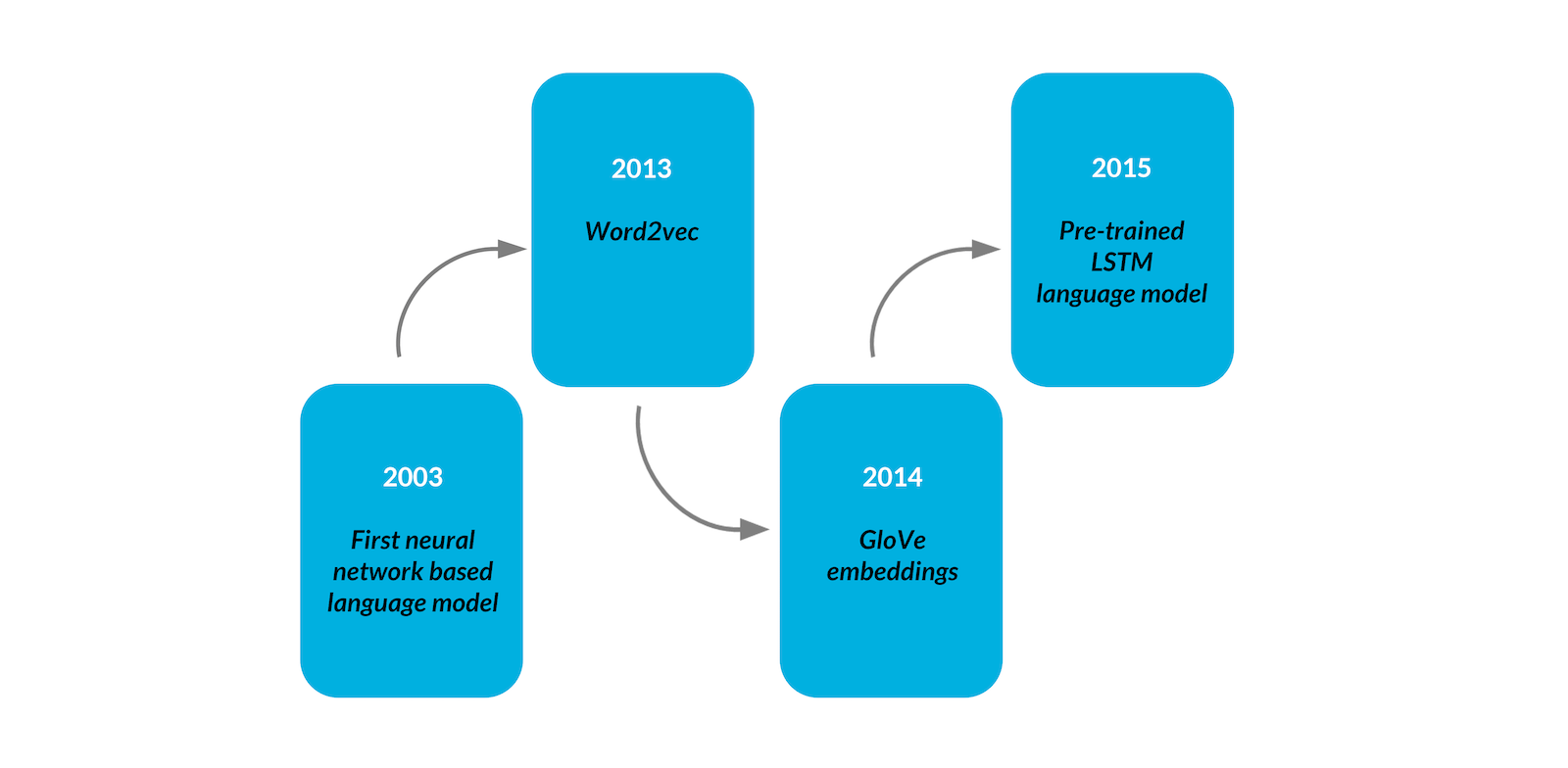
Figure 1: NLP Timeline
Since 2015, researchers have been experimenting with the idea of semi-supervised pre-training of LSTM [1] and Transformer-based language models on large corpora of text, and then supervised fine-tuning them for specific tasks on a much smaller dataset. BERT [2] and GPT-1 [3] are two examples of such approaches. Such methods eliminated the need for task-specific models, resulting in architectures that outperformed existing solutions to many difficult NLP tasks. Even though the task-specific dataset and fine-tuning were still required, it is a significant improvement.
The scarcity of large enough datasets for some tasks, the effort required to create them, and the lack of generalization of fine-tuned models outside the training distribution prompted the development of a new, human-like paradigm in which all that is required is a short natural language description of the task that the model is asked to perform, with an optional, tiny number of demonstrations added to the instruction. GPT-2 [4], GPT-3 [5], and other generative language models described in the following section represent this paradigm.
GPT is an abbreviation of Generative Pre-trained Transformer. It is generative in the sense that it can generate text-given input. Because it has already been trained on a large corpus of text, it is pre-trained. Finally, it is a neural network architecture that is based on the Transformer [6].
A GPT generates text in response to a text input, called a prompt. It is a simple but versatile framework, as many problems can be converted to text-to-text tasks. On the one hand, GPT can be asked to perform standard NLP tasks such as summarizing/classifying a text passage, answering questions about a given piece of text, or extracting named entities from it. On the other hand, due to its generative nature, GPT is an ideal tool for creative applications. It can create a story based on a brief premise, hold a conversation, or… write a blog post. Furthermore, if trained on a corpus of code, such a model could perform code generation, editing, and explanation tasks, such as generating Python docstrings, generating git commit messages, translating natural language to SQL queries, or even translating code from one programming language to another.
Modern language models, such as OpenAI’s GPT-3, Google’s LaMDA [7], and DeepMind’s Gopher [8], are essentially GPT implementations. They are much more powerful than the original GPT-1, mostly because of their size – for instance, the largest variant has 175 billion parameters – and because they were pre-trained on massive amounts of text; in the case of GPT-3, it was hundreds of billions of words.
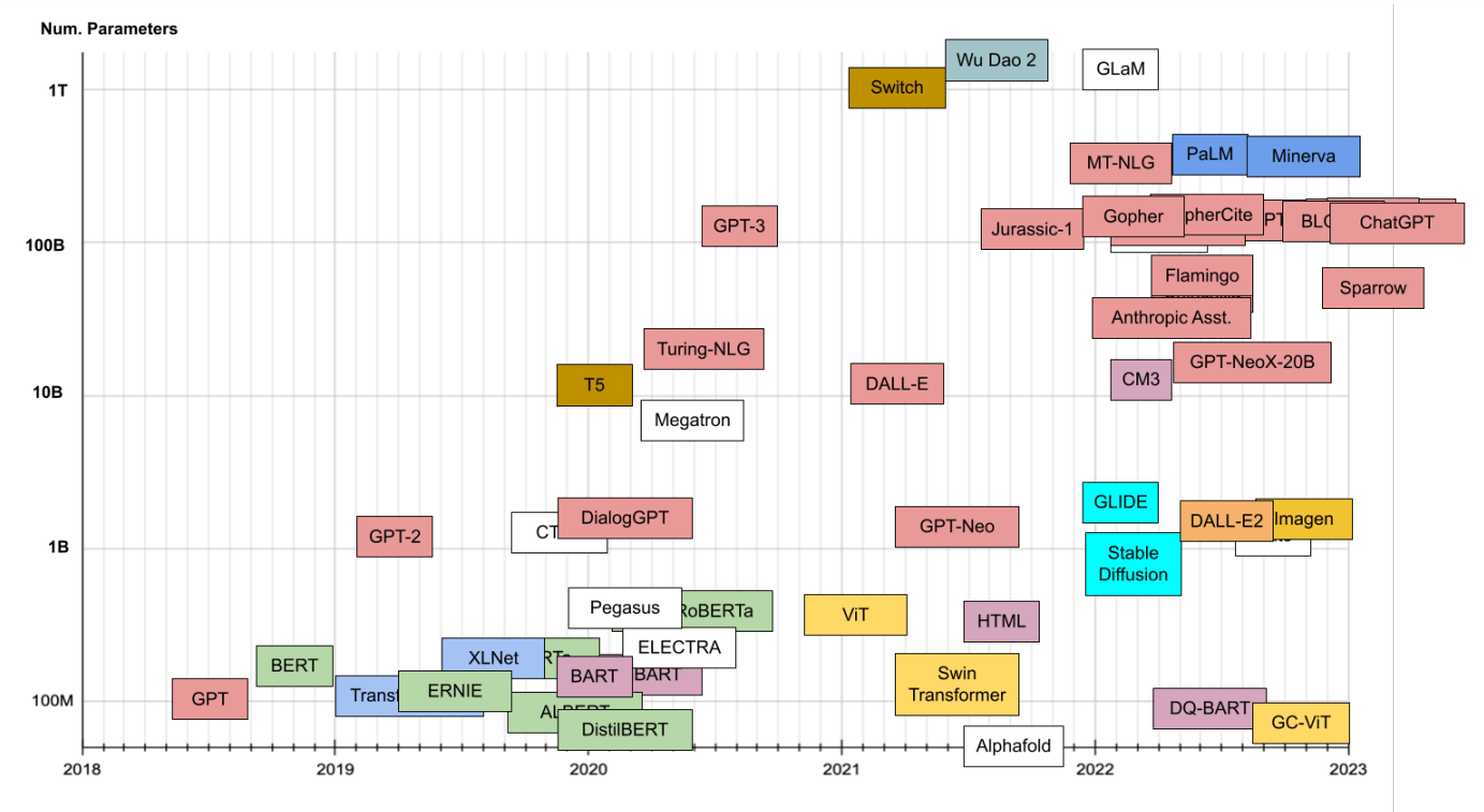
Figure 2: Number of parameters and the release date of Transformer-based models. GPT-like models are highlighted in red. Source: [9]
From a technical standpoint, the model is a decoder-only variant of a Transformer model, consisting of a stack of Transformer blocks followed by a linear layer and softmax that predict the probability that each word in the model’s vocabulary is the next token in a sequence. Each transformer block is composed of a Multi-Head Casual Self Attention layer, a linear layer, layer normalizations, and residual connections. This architecture can be thought of as a “general-purpose differential computer” that is both efficient (transformers enable high parallelism of computation) and optimizable (via backpropagation)[10].
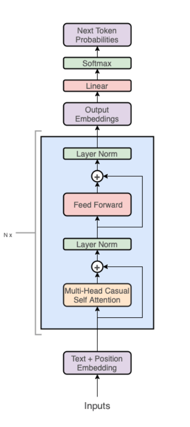
Figure 3: Decoder architecture underpinning the GPT-like models Source: [11]
The research community recently took a few steps forward in the development of language models. GPT-family models are trained to complete the input text rather than follow the user’s instructions. To make the models generate more sensible outputs in response to user instructions, as well as to make them more truthful and less toxic, the authors opted for the inclusion of human feedback in the process of training the model. This technique, called Reinforcement Learning from Human Feedback (RLHF) is so interesting that we decided to devote a whole blog post to describing it in detail – feel free to read more about it here!
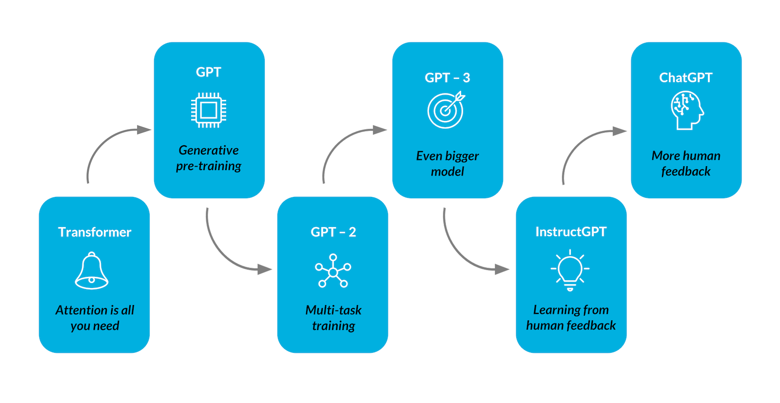
Figure 4: Evolution from transformer architecture to ChatGPT
The application of this technique has resulted in new iterations of the models, such as InstructGPT [12] and ChatGPT [13]. The latter was the subject of massive attention from the public, even outside of the AI world itself. ChatGPT created a stir in the media, mostly because of its availability and API that allows everyone to use it directly [14].
With just a couple of commands, ChatGPT can prove its ability to interact with a human by producing a well-tailored resume, playing a game of chess, or writing a part of compilable code. It also acts as an information distiller, providing a comprehensive yet concise summary of a given subject.
OpenAI recently enabled ChatGPT API access under the name gpt-3.5-turbo. It’s a GPT-3.5 model optimized for the chat that costs one-tenth the price of the best previously available model. More information on that can be found here.
Future perspectives
In spite of the fact that such developments are clearly ground-breaking, there seems to be a long way to go for it to become standard for general NLP purposes. Current studies prove that even though the model is impressive given its do-it-all ability, it is underperforming compared to existing state-of-the-art solutions for NLP tasks. For instance, in the recently published paper by J. Kocon et al., ChatGPT seems to be yielding worse results than the current best models in all of the 25 different NLP tasks that were tested in the publication [15]. Anyone who has used the model for a bit longer could notice its limitations, such as the fact that it lacks knowledge of recent events.
We are eager to observe further development in this area of AI. Ideas to make the model better and more versatile seem to be never-ending and the results are already looking very promising.
Bibliography
United States of America
Poland