How to train a Large Language Model using limited hardware?
Large language models (LLMs) are yielding remarkable results for many NLP tasks, but training them is challenging due to the demand for a lot of GPU memory and extended training time. This is compounded by the fact that the size of many models exceeds what a single GPU can store. For instance, to fine-tune BLOOM-176B, one would require almost 3 TB of GPU memory (approximately 72 80GB A100 GPUs). In addition to the model weights, the cost of storing intermediate computation outputs (optimizer states and gradients) is typically even higher. To address these challenges, various parallelism paradigms have been developed, along with memory-saving techniques to enable the effective training of LLMs. In this article, we will describe these methods.
Data parallelism
In data parallelism (DP), the entire dataset is divided into smaller subsets, and each subset is processed simultaneously on separate processing units. During the training process, each processing unit calculates the gradients for a subset of the data, and then these gradients are aggregated across all processing units to update the model’s parameters. This allows for the efficient processing of large amounts of data and can significantly reduce the time required for training deep learning models.
While data parallelism can offer significant benefits in terms of reducing the time taken to train deep learning models, there are also several constraints associated with this technique. The key constraint of data parallelism is that each processing unit needs to store a copy of the entire model’s parameters and gradients, which can be a significant memory overhead. Naive DP cannot work well if the model size is larger than the memory of a single GPU node. Later in this article, we will elaborate on how to work with limited GPU memory when the model is too big to fit on one machine.Pipeline Parallelism
Since deep neural networks typically have multiple layers stacked on top of each other, the naive approach to model parallelism involves dividing a large model into smaller parts, with a few consecutive layers grouped together and assigned to a separate device, with the output of one stage serving as the input to the next stage. For instance, if a 4-layer MLP is being parallelized across 4 devices, each device would handle a different layer. The output of the first layer would be fed to the second layer and so on, until the last layer’s output is produced as the MLP’s output.

Figure 2: The naive model parallelism strategy is inefficient because the network works in a sequential manner and can only use one accelerator at a time. Source: [3]
To address the need for efficient pipeline parallelism, in 2019 researchers at Google introduced a new technique for parallelizing the training of deep neural networks across multiple GPUs – GPipe (Huang et al. 2019).
Unlike naive model parallelism, GPipe splits the layers in a way that maximizes parallelism while minimizing communication between GPUs. The key idea behind GPipe is to partition theincoming batch into smaller micro-batches, which are processed in a distributed manner on the available GPUs. The GPipe paper found that if there are at least four times as many microbatches as partitions, the bubble overhead is almost non-existent. Furthermore, the authors of the paper report that the Transformer model exhibits an almost linear speedup when the number of microbatches is strictly larger than the number of partitions.

Figure 3: GPipe splits the input mini-batch into micro-batches, which can be processed by multiple accelerators at the same time. Source: [3]
However, when a single parameter, such as a large embedding table with a large vocabulary size, requires a significant amount of GPU memory, the methods described in this paragraph become inefficient since treating this large tensor as an atomic unit impedes the balance of the memory load.
Tensor Parallelism
In tensor parallelism, specific model weights, gradients and optimizer states are split across devices and each device is responsible for processing a different portion of the parameters.
In contrast to pipeline parallelism, which splits the model layer by layer, tensor parallelism splits individual weights. In this section we will describe the technique for parallelizing a Transformer model with tensor parallelism using an approach that was proposed in the Megatron-LM paper (Shoeybi et al. 2020).
A Transformer layer consists of a self-attention block followed by a two-layer perceptron. First, we will explain the MLP block.
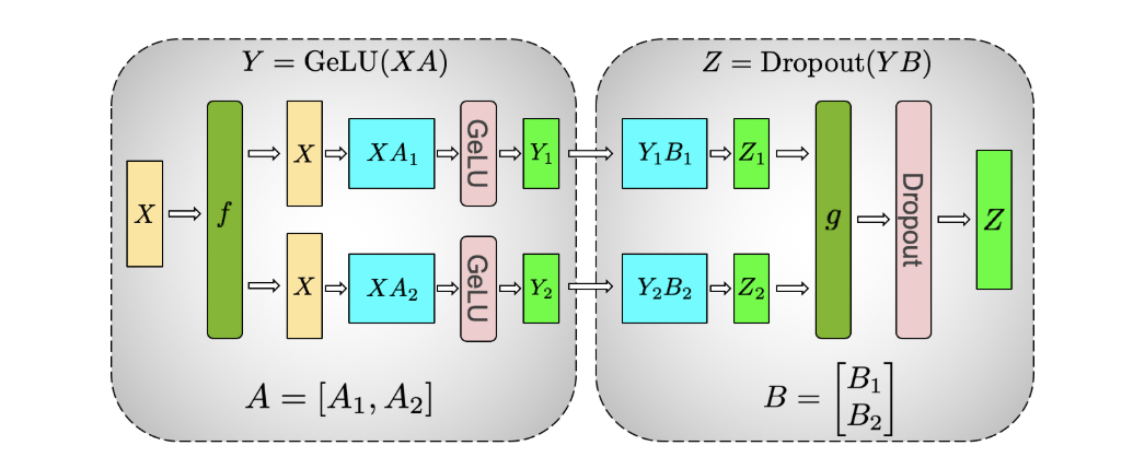
Figure 4: Illustration of tensor parallelism for the MLP block. Source: [5]
The first part of the block is a GEMM (General Matrix Multiplication) operation followed by a GeLU. The GEMM operation is partitioned in such a way that the weight matrix \(A\) is split along its columns \(A=[A_1, A_2]\) and GeLU can be independently applied to the output of each partitioned GEMM:
$$
[Y_1, Y_2] = [GeLU(XA_1), GeLU(XA_2)].
$$
In this way, a synchronization point can be skipped. The second GEMM operation is performed such that the weight matrix \(B\) is split along its rows and input \(Y\) along its columns:
$$
Y = [Y_1, Y_2], B = [B_1, B_2]^T,
$$
resulting in \(Z = Dropout(YB) = Dropout(Y_1B_1 + Y_2B_2)\).
We will now move on to the explanation of the self-attention block.
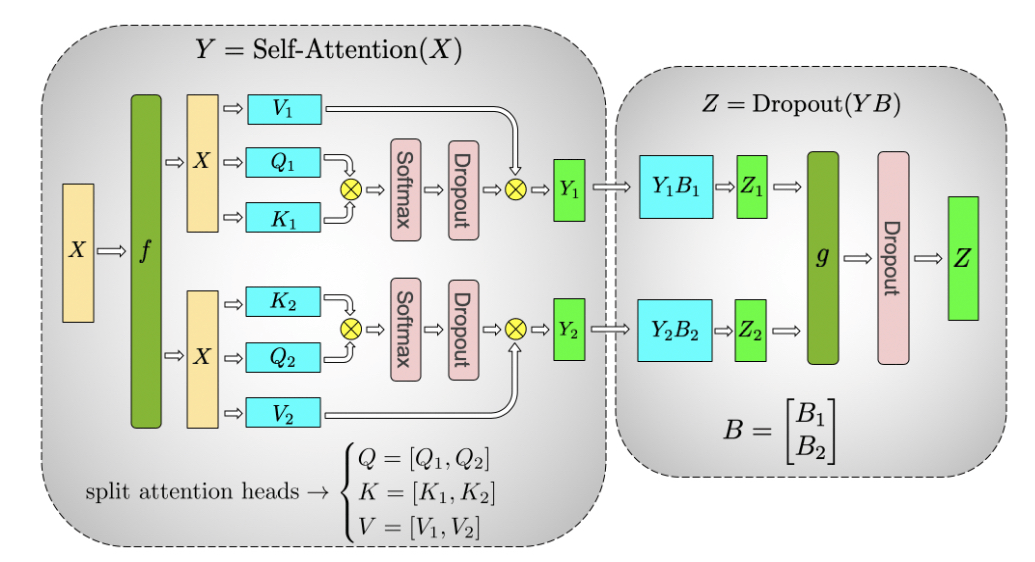
Figure 5: Illustration of tensor parallelism for the self-attention block. Source: [5]
It runs GEMM with query (\(W^Q\)), key (\(W^K\)), and value weights (\(W^V\)) according to the previously explained partitioning in parallel. Next, another GEMM is used to produce the attention head results:
$$
Attention(Q, K, V) = softmax \big( \frac{QK^T}{\sqrt{d_k}} \big) V.
$$
To measure the scalability of their implementation, the authors of the MegatronLM paper considered GPT-2 models with \(1.2, 2.5, 4.2\) and \(8.3\) billion parameters. They evaluated both tensor parallelism and a combination of tensor parallelism with 64D data parallelism which demonstrated up to 76% scaling efficiency using 512 GPUs. Mixed Precision Training and Activation Checkpointing techniques were also used – we elaborate more in the following paragraphs.
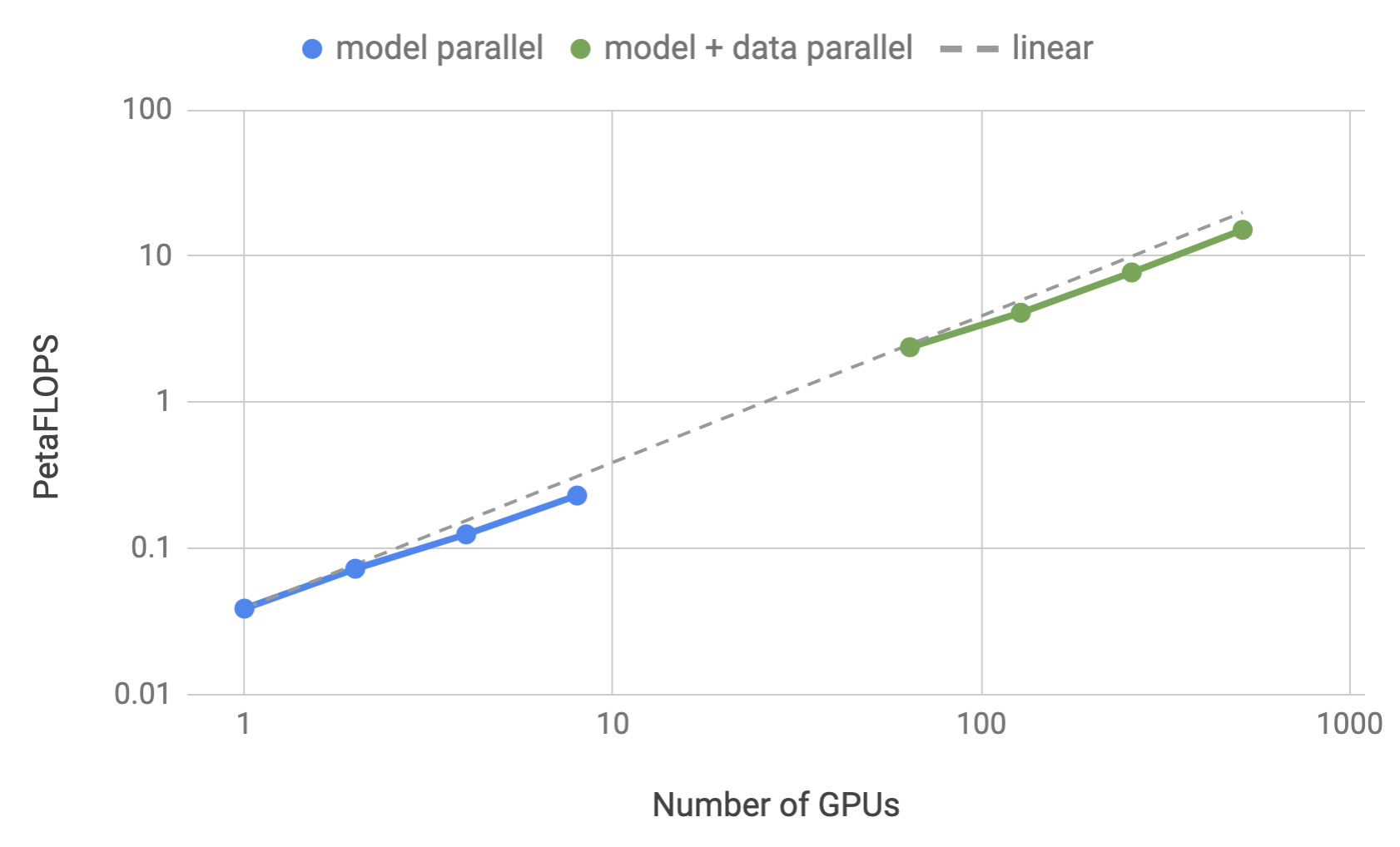
Figure 6: Training efficiency for tensor parallelism and a combination of tensor parallelism with data parallelism as a function of the number of GPUs. Source: [5]
Sequence parallelism
Another method to parallelize computation across multiple devices is Sequence Parallelism (Li et al. 2021), a technique for training Transformer models on very long sequences by breaking them up into smaller chunks and processing each chunk in parallel across multiple GPUs.
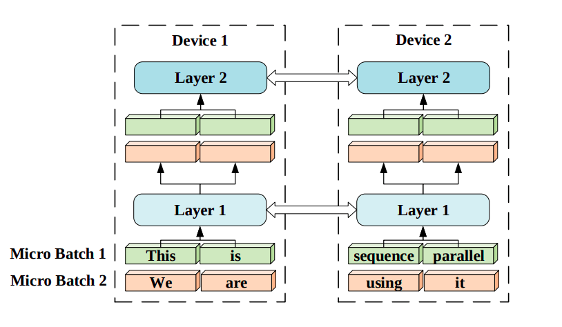
Figure 7: Sequence parallelism illustration. Input sequences are divided into smaller pieces and distributed to corresponding devices. Each device has the same trainable parameters but different sub-sequence input chunks. Source: [7]
The main challenge in this approach is computing attention scores across devices. To solve this problem, the authors came up with a new method called Ring Self-Attention (RSA), which makes it possible to compute attention scores in a distributed setting. There are two steps in RSA which we will briefly describe in this section.
We begin by establishing some notations which we adopt from the original paper. We assume that the embeddings on the n-th device correspond to the n-th chunk of the input sequence and are denoted as \(K^n\) (key), \(Q^n\) (query), and \(V^n \) (value). Additionaly, we set the number of available GPUs to \(N\).
The goal of the first stage of RSA is to compute \(Attention(Q^n, K, V)\) which is the self-attention layer output on the n-th device. To achieve this, the key embeddings are shared among the devices and used to calculate attention scores \(QK^T\) in a circular manner. This requires \(N-1\) rounds of communication. As a result, all attention scores \(S^1, S^2, \dots, S^N\) are stored on the proper devices.
In the second stage of RSA, the self-attention layer outputs \(O^1, O^2, \dots, O^N\) are calculated. For this purpose, all value embeddings are transmitted in a similar way as the key embeddings in the previous stage.
Mixture-of-Experts
The fundamental concept behind the Mixture-of-Experts method (MoE, Shazeer et al. 2017) is ensemble learning. To go into more detail, the MoE layer consists of a set of \(n\) feed-forward expert networks \(E_1, E_2, \dots, E_n\) (which can be distributed across GPUs) and the gating network \(G\) whose output is a sparse \(n\) -dimensional vector. The output \(y\) of the MoE layer for a given input \(x\) is
$$
y = \sum\limits^{n}_{i=1} G(x)_i E_i(x),
$$
where \(G(x)\) denotes the output of the gating network and \(E_i(x)\) – the output of the \(i\)-th expert network. It is easy to observe that wherever \(G(x)_i = 0\) there is no need to evaluate \(E_i\) on \(x\).
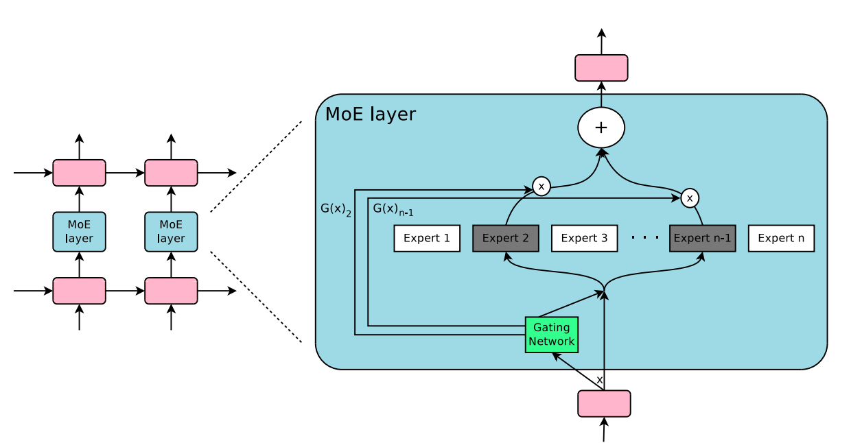
Figure 8: Illustration of a mixture-of-experts (MoE) layer where the gating network activates only two of the experts. Source: [8]
For the gating network, the authors introduced a mechanism called Noisy Top-k Gating that adds two components to the standard Softmax gating network – noise and sparsity. More precisely, before applying the softmax function, Gaussian noise is added to the input, then only the top k values are kept and the rest are set to \(– \infty\):
$$
G(x) = Softmax(KeepTopK(H(x), k))
$$
$$
H(x)_i = (x \cdot W_g)_i + \epsilon \cdot softplus((x \cdot W_{noise})_i), \epsilon \sim N(0, 1),
$$
$$
KeepTopK(v, k)_i = v_i \mbox{ if } v_i \mbox{ is in the top } k \mbox{ elements of } v, -\infty \mbox{ otherwise }.
$$
Activation Checkpointing
Suppose we partition a neural network into k partitions. In Activation Checkpointing (Chen et al. 2016), only the activations at the boundaries of each partition are saved and shared between workers during training. The intermediate activations of the neural network are recomputed on-the-fly during the backward pass of the training process rather than storing them in memory during the forward pass.
Mixed Precision Training
Two common floating-point formats used in Deep Learning applications are the single-precision floating-point format (FP32) and the half-precision floating-point format (FP16). The half-precision data type uses 16 bits to represent a floating-point number, with 1 bit for the sign, 5 bits for the exponent, and 10 bits for the significand. On the other hand, FP32 uses 32 bits, with 1 bit for the sign, 8 bits for the exponent, and 23 bits for the significand.

Figure 9: FP16 and FP32 formats. Source: [16]
The main advantage of using FP16 over FP32 is that it requires only half as much memory,
which can be beneficial in applications where speed and reduced memory usage are more important than accuracy, such as in Deep Learning models that require a large number of calculations. However, FP16 is less precise than FP32, which means that it can result in rounding errors when performing calculations.
The concept of Mixed Precision Training (Narang & Micikevicius et al. 2018) bridges the gap between reducing memory usage during training and maintaining good accuracy.
Mixed Precision Training involves utilizing FP16 to store weights, activations, and gradients. However, to maintain accuracy similar to that of FP32 networks, an FP32 version of the weights (the master weights) is also kept and modified using the weight gradient during the optimizer step. In each iteration, a copy of the master weights in FP16 is utilized in both the forward and backward passes, which reduces storage and bandwidth requirements by half compared to FP32 training.
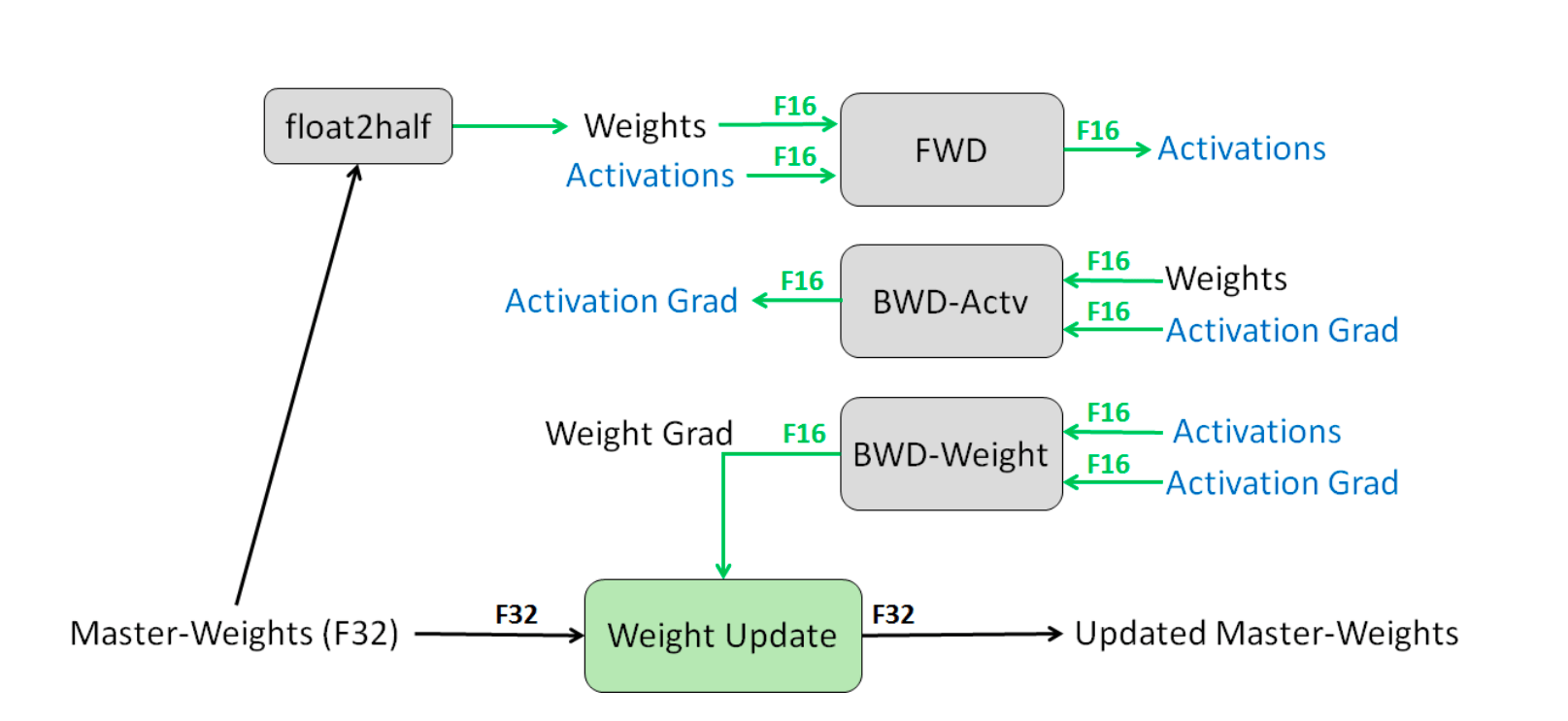
Figure 10: Mixed precision training process. Source: [9]
When using FP16, the range of representable values is smaller than when using FP32, which can cause the gradients to become very small and ultimately disappear. This can make it difficult to train a deep neural network effectively.
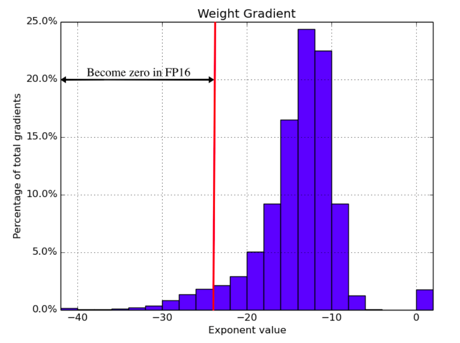
Figure 11: The distribution of weight gradient exponents when training a speech recognition model with FP32 weights. Source: [9]
To better handle gradients with small magnitudes, loss scaling is used. In loss scaling, the loss function is multiplied by a scaling factor before computing the gradients during backpropagation. This scaling factor increases the magnitude of the gradients, thereby preventing them from becoming too small and underflowing. Finally, the gradients are divided by the same scaling factor to undo the scaling, and used to update the weights.
The authors of “Mixed Precision Training” also provide experimental results showing the effectiveness of the technique on image classification and language translation tasks. In both cases, Mixed Precision Training matched the FP32 results.
Zero Redundancy Optimizer
Optimizers use a lot of memory. For example, while using the Adam optimizer, we need to save four times the memory of model weights, as it stores momentums and variances which are as big as the gradients and model parameters (Weng 2021).
All parallelism techniques described in the previous sections store all the model parameters required for the entire training process, even though not all model states are needed during training. To address these drawbacks of training parallelism while retaining the benefits, Microsoft researchers developed a new memory optimization approach called Zero Redundancy Optimizer (ZeRO, Rajbhandari et al. 2019).
ZeRO aims to train very large models efficiently by eliminating redundant memory usage, resulting in better training speed. It eliminates memory redundancies in Data Parallel processes by dividing the model states across the devices instead of duplicating them.
ZeRO has three optimization stages:
- Optimizer Partitioning: The optimizer state is divided equally among available devices. Each GPU only stores and updates its assigned optimizer state and parameters during training.
- Gradient Partitioning: Only gradients responsible for updating corresponding parameters in the assigned partitions are sent to the GPU during backpropagation.
- Parameter Partitioning: Only the partition of a parameter needed for forward and backward propagation is stored in the GPU. Other required parameters are received from other GPUs.
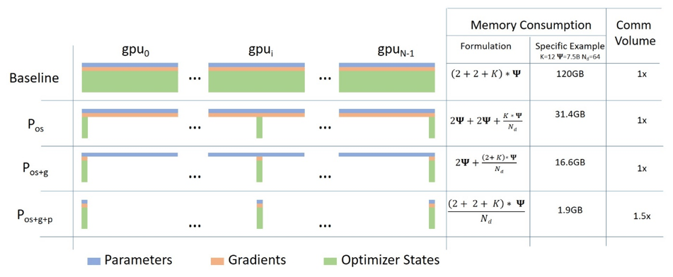
Figure 12: Three optimization stages of ZeRO compared with the data parallelism baseline. Source: [13]
According to the authors, memory reduction is directly proportional to the degree of data parallelism. For instance, partitioning across 8 GPUs will lead to an 8-fold reduction in memory usage.
FlashAttention
Making Transformers understand longer inputs is difficult because their multi-head attention layer needs a substantial amount of memory and time to process the input, and this requirement grows quadratically with the length of the sequence. When training Transformers on long sequences with parallelism techniques described in previous sections, the batch size can become extremely small. This is the scenario which the FlashAttention method (Dao et al. 2022) improves.
To optimize for long sequences for each attention head, FlashAttention splits the input \(Q, K, V\) into blocks and loads these blocks from GPU HBM (which is the main memory) into SRAM (which is its fast cache). Then, it computes attention with respect to that block and writes back the output to HBM.
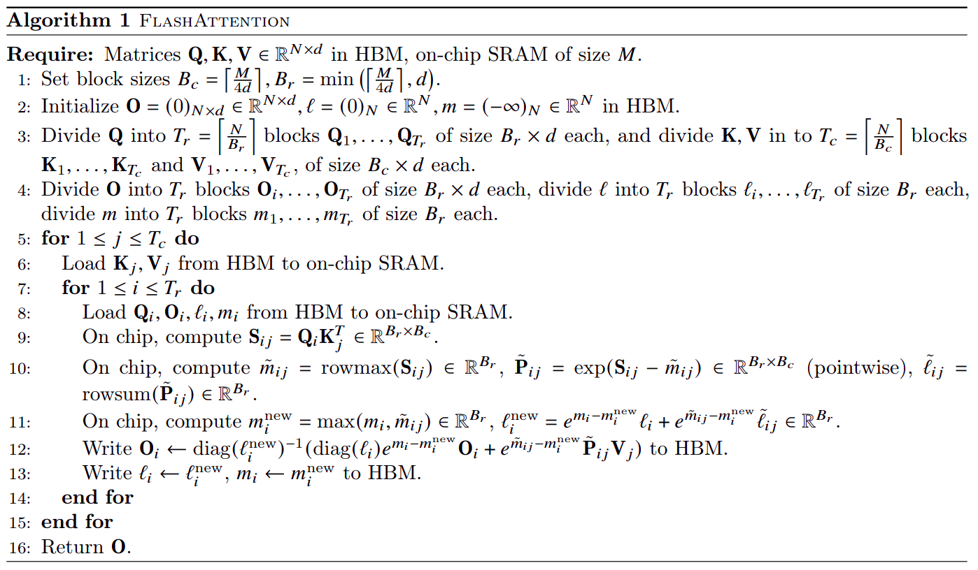
Figure 13: FlashAttention algorithm. Source: [14]
In further research (Dao 2023), the author additionally parallelizes over the sequence length dimension. It is reported that while keeping the number of heads at 12 and head dimension at 128 and using an A100 40GB GPU, FlashAttention is between 2.2x and 2.7x faster for longer sequences (8k) compared to Pytorch and Megatron-LM attention implementations.
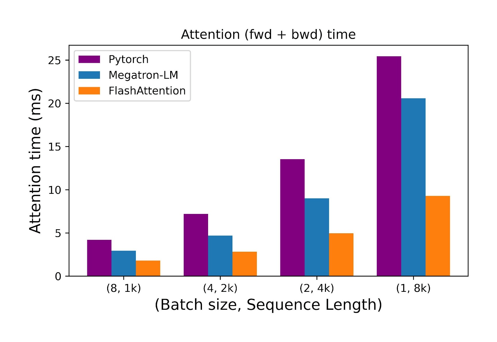
Figure 14: Comparison of the time taken by the forward and backward passes of the attention layer as the sequence length increases while the batch size decreases. Source: [15]
Also, in the case of end-to-end training, a significant speed-up was obtained. The usage of FlashAttention to train Transformers of up to 2.7B parameters on sequences of 8k in length made training 2.2 times faster compared to Megatron-LM.
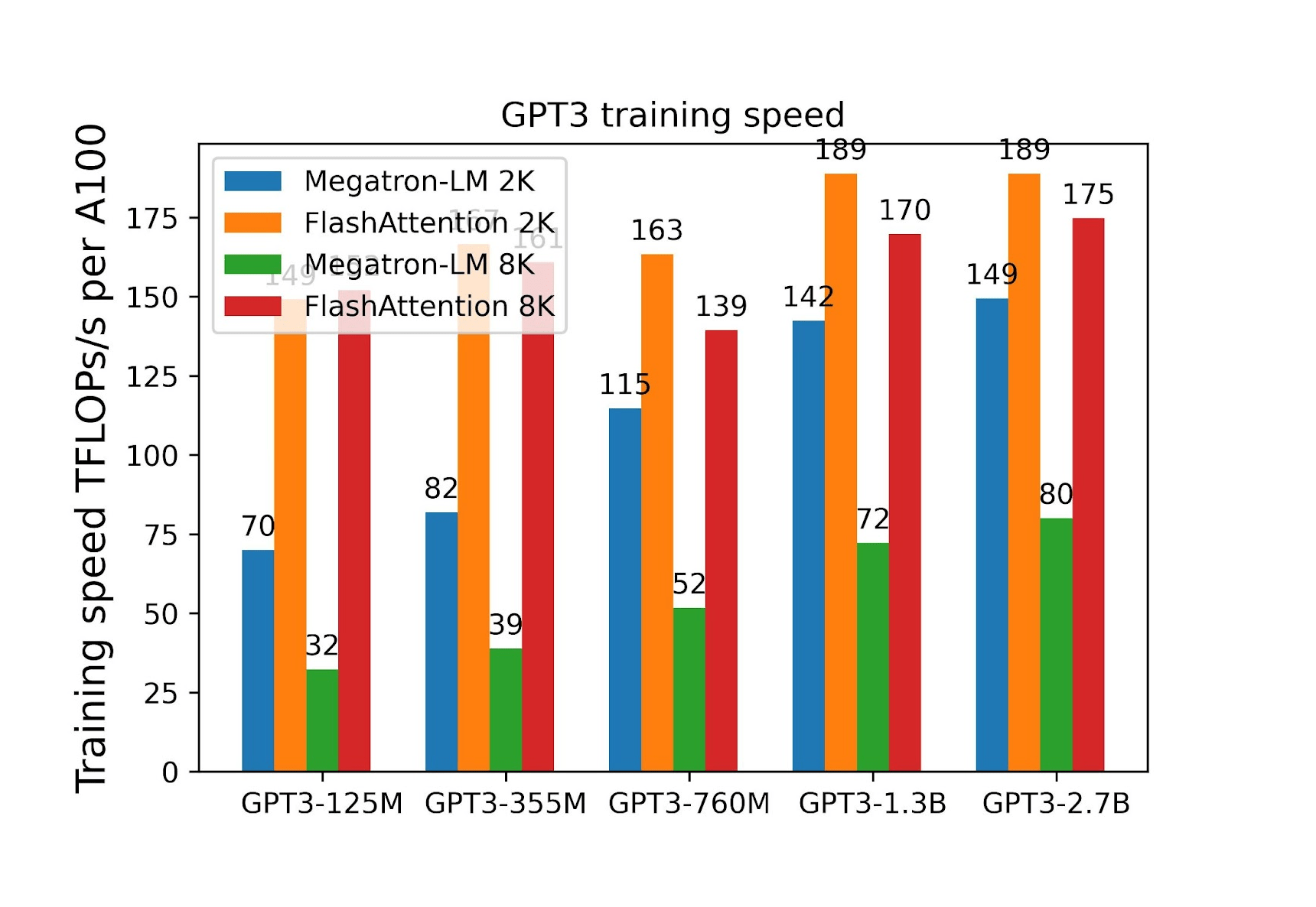
Figure 15: Training efficiency as a function of the model size. Source: [15]
How to train Large Language Models: final thoughts
In the article, various memory optimization techniques for training large language models were discussed. We explained different parallelism paradigms: Data Parallelism, Naive Model Parallelism, Pipeline Parallelism, Tensor Parallelism and Sequence Parallelism. In addition, some pros and cons of these approaches were presented. We then moved on to other memory optimization methods: Mixture-of-Experts, Mixed Precision Training and ZeRO (Zero Redundancy Optimizer). While explaining Mixed Precision Training, we also went through the Loss Scaling technique. Finally, we introduced FlashAttention – an algorithm dedicated to memory reduction for the attention layer.
To sum up, we’ve presented several methods that it’s important to be familiar with when training large language models, as these methods can help improve the efficiency, scalability, and cost-effectiveness of the training, as well as optimizing resource utilization.
Are you ready to explore the potential of large language models like GPT? Join our GPT and other LLMs Discovery Workshop to start your AI journey today.
References
- Petals: Collaborative Inference and Fine-tuning of Large Models, Alexander Borzunov et al. 2022
- How to train really large models on many GPUs?, Lilian Weng 2021
- GPipe: Efficient Training of Giant Neural Networks using Pipeline Parallelism, Huang et al. 2019
- Tensor Parallelism, Amazon SageMaker Documentation 2023
- Megatron-LM: Training Multi-Billion Parameter Language Models Using Model Parallelism, Shoeybi et al. 2020
- Training Deep Nets with Sublinear Memory Cost, Chen et al. 2016
- Sequence Parallelism: Long Sequence Training from System Perspective, Li et al. 2021
- Outrageously Large Neural Networks: The Sparsely-Gated Mixture-of-Experts Layer, Shazeer et al. 2017
- Mixed Precision Training, Narang & Micikevicius et al. 2018
- Train With Mixed Precision, NVIDIA Docs Hub 2023
- NeMo Megatron, NVIDIA NeMo 2022
- ZeRO: Memory Optimizations Toward Training Trillion Parameter Models, Rajbhandari et al. 2019
- ZeRO & DeepSpeed: New system optimizations enable training models with over 100 billion parameters, DeepSpeed Team, Rangan Majumder & Junhua Wang 2020
- FlashAttention: Fast and Memory-Efficient Exact Attention with IO-Awareness, Dao et al. 2022
- FlashAttention: Fast Transformer training with long sequences, Dao 2023
- The bfloat16 numerical format, Cloud TPU Documentation 2023


