How to perform self-supervised learning on high-dimensional data
In this post, the self-supervised learning paradigm is discussed. This method of training machine learning models is emerging nowadays, especially for high-dimensional data. In order to focus the attention of this article, we will only work on examples from the computer vision area. However, the methods presented are general and may be successfully used for problems from other domains as well.
Introduction
As data sets grow and tasks become more complicated, supervised learning and reinforcement learning approaches turn out to be harder to apply efficiently. The reason is that the feedback signal needed during training is becoming increasingly hard to obtain.
In this post, I present another learning paradigm which is free of this problem – self-supervised learning. This method of training machine learning models is emerging nowadays, especially for high-dimensional data.
In order to focus the attention of this article, we will only work on examples from the computer vision area. However, the methods presented are general and may be successfully used for problems from other domains as well.
The challenge of labeling in supervised learning and reinforcement learning
Current deep learning techniques work great in tasks where there is plenty of data that comes with a feedback signal. In supervised tasks, the feedback comes in the form of error signals computed based on the labels attached to each data point. Thus, we have to specify the correct output for a given input.
In reinforcement learning, a scalar feedback signal is provided from the environment. In this case we do not have to state how the agent should behave, but we should be able to assess how the agent has performed. This is usually done in the context of tasks that have a temporal aspect — the AI agent acting in its environment over multiple time steps must adjust its behavior based on possibly delayed and sparse reward signals.
The problem with the supervised approach is that it does not scale very well. It may be relatively easy to label 100 images, but usually we need thousands or millions of labeled examples before the model can learn the nuances of the task. All practitioners can probably confidently say that there are hardly ever enough labeled data points.

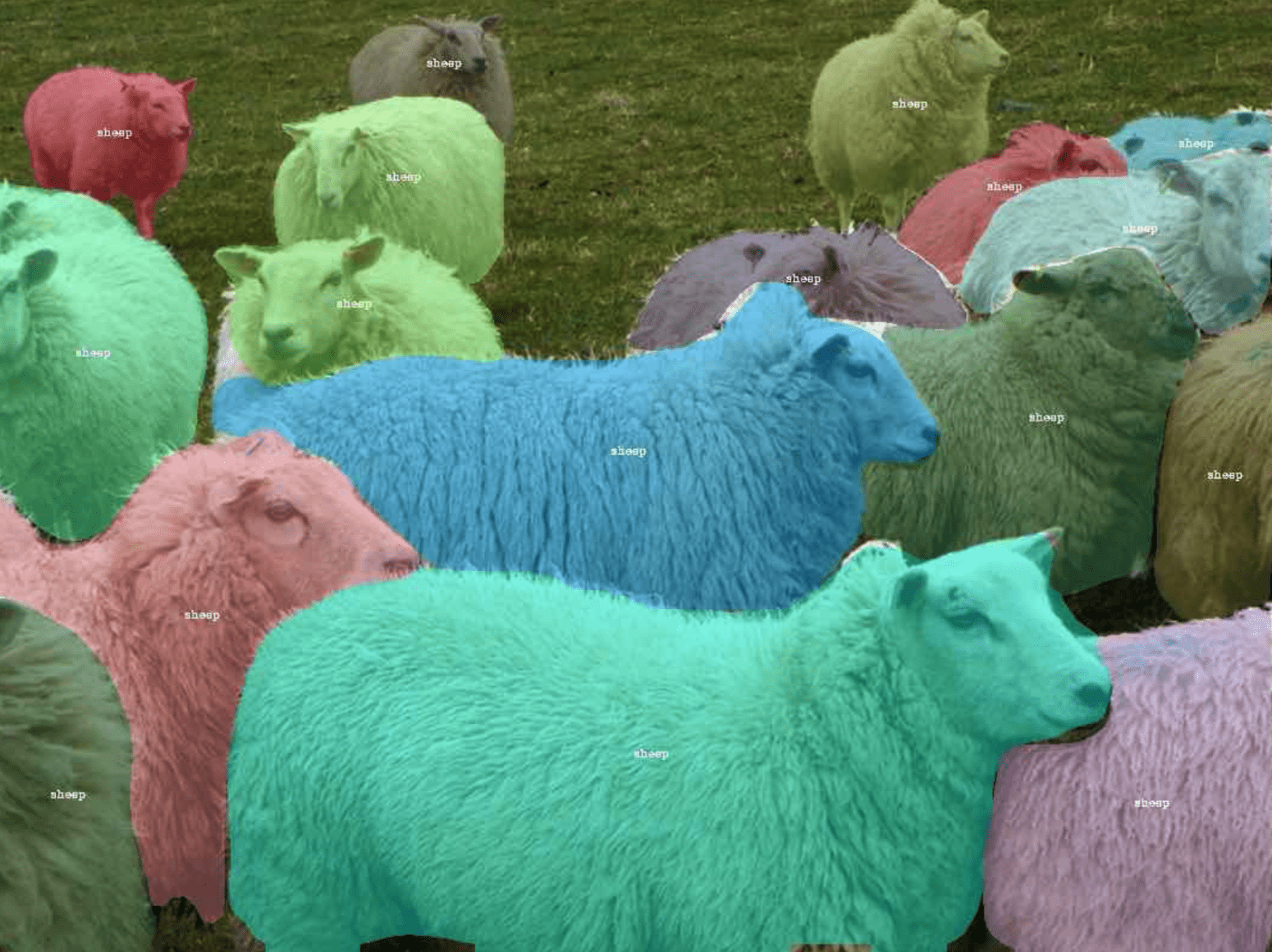
Source: SOLO paper. If we want to train a good model to segment sheeps using supervised learning, we have to color every single sheep manually in hundreds of pictures.
In the context of reinforcement learning, it may be relatively easy to obtain many samples (episodes) from virtual environments, like with chess, Go, or Atari games. However, this is becoming much more difficult in the “wild” with an actual physical agent interacting with the real world. Not only is the environment richer and noisier, but it may not be feasible to obtain many episodes with bad actions (think about self-driving cars or AI controlling nuclear power plants).
This is one of the reasons why we almost always use transfer learning. Here, we take a model that was pre-trained on another dataset (e.g., in computer vision the standard practice is to use ImageNet) and use it as a starting point for training on our dataset. Note that ImageNet is in itself a fairly large labeled dataset. But there is so much more digital data available!
Could we somehow benefit from that data without laborious and time-consuming labeling? I will try to answer this question later in this article.
Pretext tasks
In the absence of labels, we do not have any clear task that can be written in terms of a cost function. How can we then learn from data itself?
The general strategy is to define an auxiliary, pretext task that gives rise to a self-supervised learning (SSL) signal. To do so, in general we must ask the model to predict some aspects of input data, possibly given some corrupted version of that data. Perhaps the most straightforward idea is to work in the input space and to ask the model to generate part of the input tensor given an input that had this part of the input masked or replaced. Such SSL methods are known as generative methods and have been a big hit in the context of natural language processing, where the masked words (or tokens) are predicted given the context defined by the surrounding text.
Similar ideas have been developed in the context of computer vision and other modalities.
For example, deep belief networks are a generative model that jointly learns to map inputs to latent representations and to generate the same inputs given the latent representation, whereas masked autoencoders are tasked with reconstructing patches (pixels) that have been randomly masked from the input image, which is achieved given the context (non-masked pixels). Although such methods can be effective, generating images, sounds, videos, and other high-dimensional objects that feature a lot of variability is a rather difficult task. It would be great if we could come up with a simpler pretext task to achieve the same goal…
Useful representations
Wait, but what do we want to achieve anyway? As mentioned before, we want to pretrain our model on unlabeled data and then use it in other (“downstream”) tasks where available labeled data is limited. Therefore, the model should use the unlabeled data to learn something useful about that data: something that is transferable to other similar datasets.
One way of looking at this is to say that we want the model to take an input \(x\) (e.g., an image or a video clip) and output a vector \(z\) that represents the input in some useful way. Following the literature, we will refer to this vector as representation or embedding. Of course, the crucial thing here is to specify what “useful” means; in general, this will depend on the downstream task.
Fortunately, many tasks share some common features that can be utilized to assess whether a given representation is useful. Indeed, classification, detection, and segmentation tasks in computer vision or speech recognition are characterized by important invariances (e.g., I can recognize an object regardless of its position in the image) and equivariances (e.g., a detection box should encompass the entire object regardless of its position in the image). Notice that I did not specify whether the object is a dog or a pineapple — in this sense these are very general features that do not depend on many other details of the task.
Augmentations
Ok, but how can we translate invariances into good representations? The basic idea is to ensure that the representation features the desired invariances. To do so, we should first state the invariances – the easiest way of doing it is to list, in the form of a procedural definition, transformations that our desired representation should be invariant to.
These transformations can be implemented in the form of a function that takes an input \(x\) and outputs a new (possibly random) view \(x’\). Note that the same procedure is used as part of a standard supervised learning pipeline where it is referred to as data augmentation. In practice, when working with images one could for example use
In this article I focus on computer vision where input is a static image, but the same methods can be adapted to other modalities including cross-modal self-supervision with, say, videos that contain both sound and a series of images. The crucial difference in how to deal with these other inputs lies in defining a good set of augmentations.
Invariance term: squeeze representations together
The next step is to formalize our intuition described above in the form of a cost function. As a reminder, our goal is to ensure that the representation (output of the model) is invariant under our chosen set of augmentations. To this end, let us take two views of the same input image \(x^A\) and \(x^B\) and pass them through the model obtaining a pair of joint embeddings \(z^A\) and \(z^B\). Next, we calculate the cosine similarity between these two representations $$\mathrm{sim}(z^A, z^B) \equiv \cos{(\phi)} =\frac{z^A \cdot z^B}{\Vert z^A\Vert \Vert z^B \Vert}.$$ Ideally, we should have \(\phi=0\) (hence, \(\cos{\phi}=1\)), so we want to minimize the cost function of the form \(l_{sim} = -\mathrm{sim}(z^A, z^B)\) which we will call invariance or similarity cost. As usual, this cost should be averaged over all images in the batch, leading to $$\mathcal{L}_{sim} = -\frac{1}{N}\sum_{i=1}^N \mathrm{sim}(z_i^A, z_i^B)$$ As the similarity cost decreases, representations of different views of the same image are pressed together, ultimately leading to a model that produces representations that are invariant under the set of transformations used to augment our dataset. However, this alone will not work as a good representation extractor.
Collapse
It is easy to understand why the similarity cost by itself is not enough. Take the following rather boring model
$$
f(x) = z_0,
$$
which ignores the input and always outputs the same representation (say, \(z_0 = [1,1,…,1]\)). Since this is the simplest solution to the optimization problem defined by \(\mathcal{L}_{sim}\) and “everything which is not forbidden is allowed”, we can expect such undesirable solutions to appear frequently as we optimize \(\mathcal{L}_{sim}\).
This is indeed what happens and this phenomenon is called a (representation) collapse. It is useful to think about the current self-supervised learning techniques in terms of how they avoid collapse. From this perspective, there are two main categories of SSL methods: contrastive and regularization-based. Below we describe in detail two popular examples, each relatively simple but still representative of its category.
Projection head
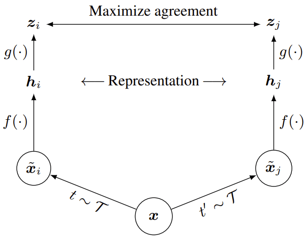
There is an additional detail: it is not actually \(z\) that is being used in downstream tasks. Instead, as it turns out, it is more beneficial to use an intermediate representation \(h\), see Fig. 1. In other words, the projection head \(g\) that is used to calculate \(z = g(h)\) is thrown away after the training. The intuition behind this trick is that the full invariance is actually detrimental in some tasks. For example, it is great if our model can report “dog” even if only the dog’s tail is visible in the image, but the same model should also be able to output “tail” or “dog tail” if it is asked to do so.

Fig. 1: A schematic diagram of a self-supervised training pipeline based on augmentations and joint embeddings. Although this image is taken from the SimCLR paper, the same overall strategy is employed in both contrastive and non-contrastive SSL methods.
Contrastive learning (SimCLR)
Contrastive learning methods can be thought of as generating supervision signals from a pretext discriminative task. In the past few years there has been an explosion of interest in contrastive learning and many similar methods have been developed. Here, let us focus on a famous example, SimCLR, which stands for “a simple framework for contrastive learning of visual representations”.
Indeed, the algorithm is pretty straightforward.
- First, take a batch of images \((x_i)_{i\in\{1,..,N\}}\) where batch size \(N\) should be large.
- Second, for a given input image \(x_k\) generate (sample) two views, \(\tilde{x}_i\) and \(\tilde{x}_j\). Note that this gives us a new, extended batch of augmented images of size \(2 N\).
- Third, apply the same base encoder \(f\) and projection head \(g\) to each sample in the extended batch obtaining “useful” representations \(h_i = f(\tilde{x}_i)\) and “invariant” representations \(z_i = g(h_i)\).
- Fourth, optimize \(f\) and \(g\) jointly by minimizing the contrastive loss \(\mathcal{L}_{InfoNCE}\).
- Last, throw away \(g\) and use \(f\) in the downstream task(s).
But what is \(\mathcal{L}_{InfoNCE}\)? In the original paper this loss function was termed NT-Xent for the “normalized temperature-scaled cross entropy loss”, but it is basically a version of InfoNCE loss introduced in the Contrastive Predictive Coding paper, which in itself is a special case of noise-contrastive estimation. The main idea here is to split the batch into positive and negative pairs. Positive pairs are two different views of the same image and, as discussed above, their representations should be close to each other. The crucial idea is that all the other (“negative”) pairs are treated as non-matching pairs whose representations should be pulled apart. Note that this approximation makes sense only if the dataset is rich enough and contains many categories. In this case the likelihood that two randomly chosen images represent the same object (or two very similar objects) is small.
How to pull negative pairs apart? In SimCLR this is achieved by the following loss
$$
\mathcal{L}_{InfoNCE} = -\frac{1}{N}\sum_{i, j=P(i)} \log\frac{\exp\left(\mathrm{sim}(z_i, z_j)\right/\tau)}
{\sum_{k\neq i}\exp\left(\mathrm{sim}(z_i, z_k)\right/\tau)},
$$
where \(P(i)\) returns the index of the other view of the same image (positive “partner”) and \(\tau\) is a “temperature” hyperparameter that is introduced to adjust how strongly hard negative examples are weighed. One can think of this loss as a cross-entropy loss for multi-class classification with a softmax layer or, in other words, as a multinomial logistic regression.
The pretext task can be then summarized as follows: given a view of an image \(\tilde{x}_i\), find the other view of the same image among the set containing all the other \(2N – 1\) views of images in the extended batch. It is also easy to see that this loss function can be decomposed as
$$
\mathcal{L}_{InfoNCE} = \mathcal{L}_{sim} + \mathcal{L}_{con},
$$
where \(\mathcal{L}_{sim}\) is the familiar similarity term discussed above
and \(\mathcal{L}_{con}\) is a contrastive term that pulls all representations in the batch apart.
Additional details:
- The base encoder can be any differentiable model. The authors of the original paper have opted for variants of ResNet-50 as this neural network has emerged as the standard architecture used to compare different methods.
- In SimCLR the projection head is a simple multilayer perceptron with a single hidden unit. The dimensionality of \(z\) does not have to be very large but it is important for the projection head to be nonlinear.
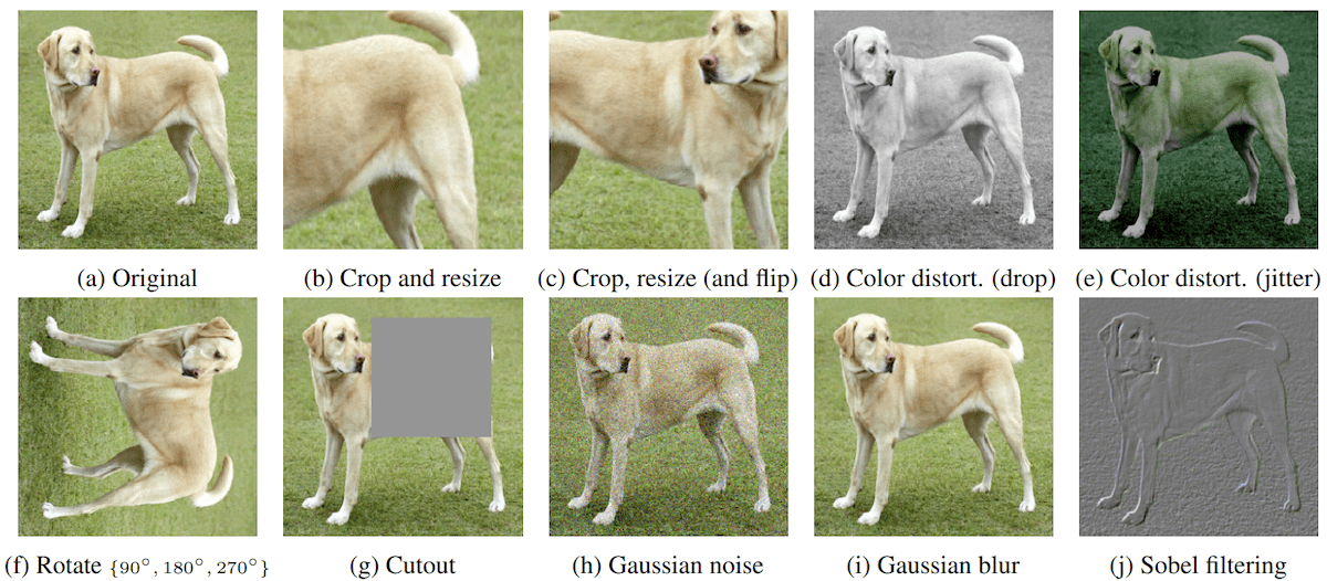
- In the original paper the authors have presented the results of systematic experiments aiming to find the best set of augmentations: see Fig. 2 that shows the augmentations studied in the paper. They found that no single transformation is enough to learn good representations. The best results among pairs of transformations were obtained by combining random cropping with random color distortion. Interestingly, the authors have also included random Gaussian blur in their standard pipeline.
- This method strongly benefits from relatively large batch sizes and long training sessions.
- Some interesting limitations of this and other contrastive methods are discussed in this paper. If many objects are present in images, the dominant object may suppress the learning of statistics of smaller objects. Similarly, easy-to-learn shared features may suppress the learning of other features.

Fig. 2: Augmentations studied in the SimCLR paper.
Noncontrastive methods (Barlow Twins)
Noncontrastive methods avoid collapse without relying on negative pairs. This class is quite diverse and includes methods such as BYOL and SimSiam, which break the symmetry between two branches that generate two views (and their representations) of input images, as well as methods based on clustering like ClusterFit or SwAV.
Another idea is to minimize the redundancy between components of \(z\). The reduction of redundancy is the cornerstone of the efficient coding hypothesis, a theory of sensory coding in the brain proposed by Horace Barlow, hence the name Barlow twins. Here, the cost function is based upon the cross-correlation matrix \(\mathcal{C}\) of size \(M\times M\), where \(M\) is the number of representation neurons (dimensionality of \(z\)). As before, two views of each image in the batch are passed through the network leading to two representations per image, \(z^A\) and \(z^B\).
Previously we have used the notation \(z_i\) to denote the representation of an image \(i\). To better understand Barlow Twins, we have to extend our notation. Let \(z_{i,\alpha}\) denote the \(\alpha\)-th component (neuron) of vector \(z_{i}\) and \(\overline{z_{\alpha}}=(1/N)\sum_{i}z_{i,\alpha}\) the batch average of that component. Each component can be z-scored (normalized) over the batch
$$
u_{i,\alpha} = \frac{z_{i,\alpha} – \overline{z_{\alpha}}}{\sqrt{\overline{z_\alpha^2}-\overline{z_{\alpha}}^2}}.
$$
The cross-correlation matrix is defined as
$$
\mathcal{C}_{\alpha\beta}
=
\overline{u^A_{\alpha} u^B_{\beta}}.
$$
Note that only positive pairs are averaged over the batch here.
The loss is then defined as
$$
\mathcal{L}_{BT}
=
\sum_{\alpha} \left( (1 – \mathcal{C}_{\alpha\alpha})^2
+
\lambda \sum_{\beta\neq\alpha} \left(\mathcal{C}_{\alpha\beta}\right)^2
\right).
$$
The contrastive term is absent from this loss and collapse is avoided due to a different mechanism, which can be understood by analyzing two terms in the Barlow Twins loss. The first, invariance term is trying to push all the diagonal terms of the cross-correlation matrix towards \(1\) (perfect correlation).
Components of \(z^A\) and \(z^B\) are perfectly correlated when \(z^A\) and \(z^B\) are identical, as desired from the invariance principle. The second, redundancy reduction term is trying to decorrelate different neurons (components of \(z\)). This has the effect of the output neurons to contain non-redundant information about the inputs, leading to non-trivial representations.
Additional details:
- Barlow Twins do not need nearly as large batch sizes as SimCLR.
- Unlike SimCLR, Barlow Twins benefit very strongly from a large dimensional output (invariant) representation \(z\).
Summary and additional reading
Self-supervised learning is here to stay to complement supervised learning and reinforcement learning whenever getting enough labels or feedback signals from the environment becomes troublesome. As we saw, the key to beneficial training in a self-supervised manner is to smartly define the pretext task and to set the loss function carefully.
For those who would like to deepen their knowledge of this topic, I recommend the blog article on self-supervised learning written by Yann LeCun and Ishan Misra.


