Is a simple linear regression able to knock spots off SVM and Random Forest?

A friend of mine took part in a project in which he had to perform future prediction of Y characteristic. The problem was that Y characteristic showed an increasing trend over time. For the purposes of this post let us assume that Y characteristic was energy demand or milk yield of cows or any other characteristic that with positive trend over time.

So, we have discussed possible approaches to this problem. As a benchmark we used the techniques that heats up processors, like the random forest and SVM. However, it turns out (and after the fact it is along intuition) that if we deal with a generally stable trend, the range of values observed in the future might be different than the range of values observed in the past. In that case techniques such as simple linear regression may give better results than the mentioned SVM and RF (which more or less look for similar cases in the past and average them).
Let us consider the following example. We have N predictors at our disposal and we want to predict development of Y characteristic. In reality it depends on only the first characteristic. We will juxtapose SVM, RandomForest, simple regression and lasso type regularised regression.
This example will be purely simulation based. We start with small random data, 100 observations and N= 25predictors (results will be similar for larger datasets). Testing set will be beyond the domain of the training set, i.e. we increase all values by +1.

library(dplyr)
library(lasso2)
library(e1071)
library(randomForest)
library(ggplot2)
# will be useful in simulations
getData <- function(n = 100, N = 25 ){
x <- runif(N*n) %>%
matrix(n, N)
# artificial out-of-domain x
x_test <- x + 1
list(x = x,
y = x[,1] * 5 + rnorm(n),
x_test = x_test,
y_test = x_test[,1] * 5 + rnorm(n))
}
# let's draw a dataset
gdata <- getData()
head(gdata$y)
# [1] -0.5331184 3.1140116 4.9557897 3.2433499 2.8986888 5.2478431
dim(gdata$x)
# [1] 100 25

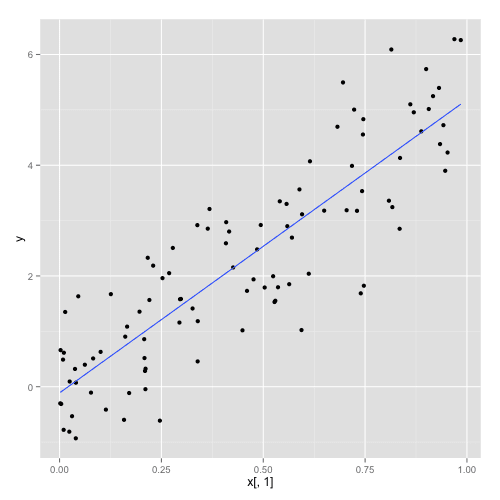
There is a linear relationships within the selected data between the first predictor and Y. We added a small random noice to avoid being too tendentious.

with(gdata,
qplot(x[,1], y) +
geom_smooth(se=FALSE, method="lm")
)

Let us fit the model for each approach and calculate MSE for each model.

fitModels <- function(x, y) {
ndata <- data.frame(y, x)
list(
model_lasso = l1ce(y ~ ., data=ndata),
model_lm = lm(y ~ ., data=ndata),
model_svm = svm(x, y),
model_rf = randomForest(x, y))
}
testModels <- function(models, x_test, y_test) {
predict_lasso <- predict(models$model_lasso, data.frame(x_test))
predict_lm <- predict(models$model_lm, data.frame(x_test))
predict_svm <- predict(models$model_svm, x_test)
predict_rf <- predict(models$model_rf, x_test)
c(
lasso = mean((predict_lasso - y_test)^2),
lm = mean((predict_lm - y_test)^2),
rf = mean((predict_rf - y_test)^2),
svm = mean((predict_svm - y_test)^2))
}
# time for fitting
models <- fitModels(gdata$x, gdata$y)
testModels(models, gdata$x_test, gdata$y_test)
# lasso lm rf svm
# 0.8425946 1.4672156 15.7713529 25.0271363

This time the Lasso wins. Now we are going to repeat random drawing and model adjustment 100 times.
And pipe this results directly to boxplots (I %)

replicate(100,{
gdata <- getData(N=N)
models <- fitModels(gdata$x, gdata$y) testModels(models, gdata$x_test, gdata$y_test) }) %>%
t() %>%
boxplot(main = paste("MSE for", N, "variables"))

The lower MSE, the better.
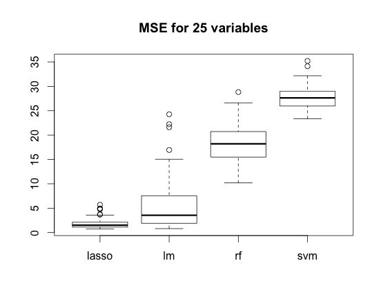
Boxplots present results of the whole simulations. We did not select the characteristics so the linear regression suffers from the random noise. Lasso regularisation helps as expected.
Of course, methods such as SVM or RandomForest must have lost that competition because in the ‘future’ value of Y is X1*5 but range of X1 is between 1-2 and not between 0-1.
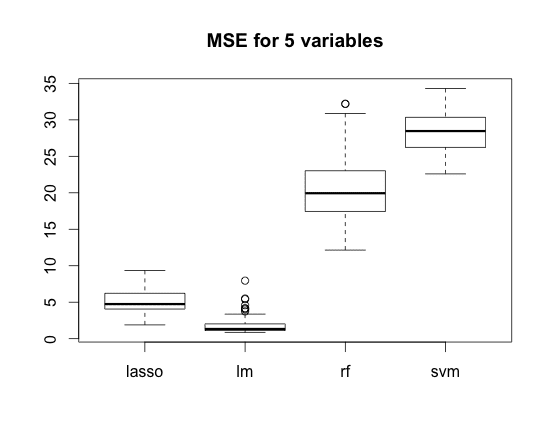
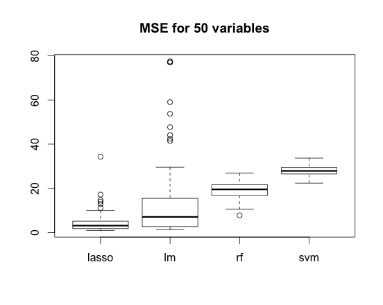
The same situation takes place in case of N=5 variables (here regression has an advantage) and N=50 variables (and here it has not).


What are the conclusions?
– SVM and RandomForest work in a ‘domain’. If some monotonic trend is observed and future values are likely to be far from these in training set, the trend should be removed in advance.
– If there are many variables, for regression it is advisable to do some variable selection first or optionally to choose a method that would do that for us (like Lasso for example). RF deal with this problem on it’s own.
– It is much more difficult to predict the future than the past ;)

Przemyslaw Biecek