Playing Atari on RAM with Deep Q-learning

In 2013 the Deepmind team invented an algorithm called deep Q-learning. It learns to play Atari 2600 games using only the input from the screen. Following a call by OpenAI, we adapted this method to deal with a situation where the playing agent is given not the screen, but rather the RAM state of the Atari machine. Our work was accepted to the Computer Games Workshop accompanying the IJCAI 2016 conference. This post describes the original DQN method and the changes we made to it. You can re-create our experiments using a publicly available code.

Atari games

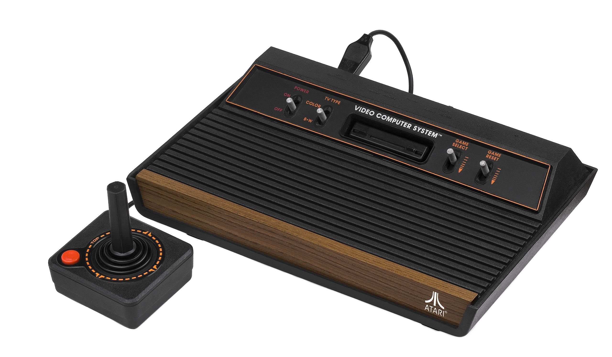
Atari 2600 is a game console released in the late 1970s. If you were a lucky teenager at that time, you would connect the console to the TV-set, insert a cartridge containing a ROM with a game and play using the joystick. Even though the graphics were not particularly magnificent, the Atari platform was popular and there are currently around \(400\) games available for it. This collection includes immortal hits such as Boxing, Breakout, Seaquest and Space Invaders.

Reinforcement Learning

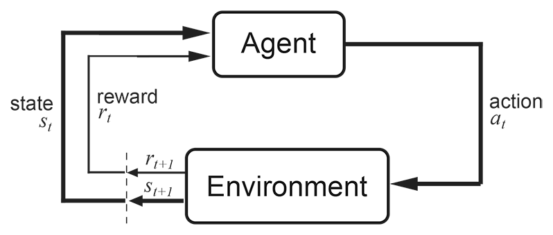
We will approach the Atari games through a general framework called reinforcement learning. It differs from supervised learning (e.g. prediction what is represented in an image using Alexnet) and unsupervised learning (e.g. clustering, like in the nearest neighbours algorithm) because it utilizes two separate entities to drive the learning:

1. agent (which sees states and rewards and decides on actions) and
2. environment (which sees actions, changes states and gives rewards).

In our case, the environment is the Atari machine, the agent is the player and the states are either the game screens or the machine’s RAM states. The agent’s goal is to maximize the discounted sum of rewards during the game. In our context, “discounted” means that rewards received earlier carry more weight: the first reward has a weight of \(1\), the second some \(gamma\) (close to \(1\)), the third \(gamma^2\) and so on.

Q-values

Q-value (also called action-value) measures how attractive a given action is in a given state. Let’s assume that the agent’s strategy (the choice of the action in a given state) is fixed. Then a Q-value of a state-action pair \((s, a)\) is the cumulative discounted reward the agent will get if it is in a state \(s\), executes the action \(a\) and follows his strategy from there on.
The Q-value function has an interesting property – if a strategy is optimal, the following holds:
$$
Q(s_t, a_t) = r_t + gamma max_a Q(s_{t+1}, a)
$$
One can mathematically prove that the reverse is also true. Namely, any strategy which satisfies the property for all state-action pairs is optimal. This fact is not restricted to deterministic strategies. For stochastic strategies, you have to add some expectation value signs and all the results still hold.

Q-learning

The above concept of Q-value leads to an algorithm learning a strategy in a game. Let’s slowly update the estimates of the state-action pairs to the ones that locally satisfy the property and change the strategy, so that in each state it will choose an action with the highest sum of expected reward (estimated as an average reward received in a given state after following given action) and biggest Q-value of the subsequent state.

for all (s,a):
    Q[s, a] = 0 #initialize q-values of all state-action pairs
for all s:
    P[s] = random_action() #initialize strategy
# assume we know expected rewards for state-action pairs R[s, a] and
# after making action a in state s the environment moves to the state next_state(s, a)
# alpha : the learning rate - determines how quickly the algorithm learns;
#                             low values mean more conservative learning behaviors,
#                             typically close to 0, in our experiments 0.0002
# gamma : the discount factor - determines how we value immediate reward;
#                               higher gamma means more attention given to far-away goals
#                               between 0 and 1, typically close to 1, in our experiments 0.95
repeat until convergence:
  1. for all s:
         P[s] = argmax_a (R[s, a] + gamma * max_b(Q[next_state(s, a), b]))
  2. for all (s, a):
         Q[s, a] = alpha*(R[s, a] + gamma * max_b Q[next_state(s, a), b]) + (1 - alpha)Q[s, a]

This algorithm is called Q-learning. It converges in the limit to an optimal strategy. For simple games like Tic-Tac-Toe, this algorithm, without any further modifications, solves them completely not only in theory but also in practice.

Deep Q-learning

Q-learning is a correct algorithm, but not an efficient one. The number of states which need to be visited multiple times to learn their action-values is too big. We need some form of generalization: when we learn about the value of one state-action pair, we can also improve our knowledge about other similar state-actions.
The deep Q-learning algorithm uses the convolutional neural network as a function approximating the Q-value function. It accepts the screen (after some transformations) as an input. The algorithm transforms the input with a couple of layers of nonlinear functions. Then it returns an up to \(18\) dimensional vector. Entries of the vector denote the approximated Q-values of the current state and each of the possible actions. The action to choose is the one with the highest Q-value.
Training consists of playing the episodes of the game, observing transitions from state to state (doing the currently best actions) and rewards. Having all this information, we can estimate the error, which is the square of the difference between the left- and right-hand side of the Q-learning property above:
$$
error = (Q(s_t, a_t) – (r_t + gamma max_a Q(s_{t+1}, a)))^2
$$
We can calculate the gradient of this error according to the network parameters and update them to decrease the error using one of the many gradient descent optimization algorithms (we used RMSProp).

DQN+RAM

In our work, we adapted the deep Q-learning algorithm so that its input are not game screens, but the RAM states of the Atari machine. Atari 2600 has only \(128\) bytes of RAM. On one hand, this makes our task easier, as our input is much smaller than the full screen of the console. On the other hand, the information about the game may be hard to retrieve. We tried two network architectures. One with \(2\) hidden ReLU layers, \(128\) nodes each, and the other with \(4\) such layers. We obtained results comparable (in two games higher, in one lower) to those achieved with the screen input in the original DQN paper. Admittedly, higher scores can be achieved using more computational resources and some additional tricks.

Tricks

The method of learning Atari games, as presented above and even with neural networks employed to approximate the Q-values, would not yield good results. To make it work, the original DQN paper’s authors and we in our experiments, employed a few improvements to the basic algorithm. In this section, we discuss some of them.

Epsilon-greedy strategy

When we begin our agent’s training, it has little information about the value of particular game states. If we were to completely follow the learned strategy at the start of the training we’d be nearly randomly choosing some actions to follow in the first game states. As the training continues, we’d stick to these actions for the first states, as their value estimation would be positive (and for the other actions would be nearly zero). The value of the first-chosen action would improve and we’d only pick these, without even testing the other possibilities. The first decisions, made with little information, would be reinforced and followed in the future.
We say that such a policy doesn’t have a good exploration-exploitation tradeoff. On one hand, we’d like to focus on the actions that led to reasonable results in the past, but on the other ahnd, we prefer our policies to extensively explore the state-action space.
The solution to this problem used in DQN is using an epsilon-greedy strategy during training. This means that at any time with some small probability \(varepsilon\) the agent chooses a random action, instead of always choosing the action with the best Q-value in the given state. Then, every action will get some attention and its state-action value estimation will be based on some (possibly limited) experience and not the initialization values.
We join this method with epsilon decay — at the beginning of training we set \(varepsilon\) to a high value (\(1.0\)), meaning that we prefer to explore the various actions and gradually decrease \(varepsilon\) to a small value, that indicate the preference to exploit the well-learned action-values.

Experience replay

Another trick used in DQN is called experience replay. The process of training a neural network consist of training epochs; in each epoch we pass all the training data, in batches, as the network input and update the parameters based on the calculated gradients.
When training reinforcement learning models, we don’t have an explicit dataset. Instead, we experience some states, actions, and rewards. We pass them to the network, so that our statistical model can learn what to do in similar game states. As we want to pass a particular state/action/reward tuple multiple times to the network, we save them in memory when they are seen. To fit this data to the RAM of our GPU, we store at most \(100 000\) recently observed state/action/reward/next state tuples.
When the dataset is queried for a batch of training data, we don’t return consecutive states, but a set of random tuples. This reduces correlation between states processed in a given step of learning. As a result, this improves the statistical properties of the learning process.
For more details about experience replay you can see Section 3.5 of Lin’s thesis. As quite a few other tricks in reinforcement learning, this method was invented back in 1993 – significantly before the current deep learning boom.

Frameskip

Atari 2600 was designed to use an analog TV as the output device. The console generated \(60\) new frames appearing on the screen every second. To simplify the search space we imposed a rule that one action is repeated over a fixed number of frames. This fixed number is called the frame skip. The standard frame skip used in the original work on DQN is \(4\). For this frame skip the agent makes a decision about the next move every \( 4cdot frac{1}{60} = frac{1}{15}\) of a second. Once a decision is made, it remains unchanged during the next \(4\) frames. A low frame skip allows the network to learn strategies based on a super-human reflex. A high frame skip will limit the complexity of a strategy. Hence learning may be faster and more successful whenever strategy matters over tactic. In our work , we tested frame skips equal to \(4,8\) and \(30\).

Further research

We are currently testing other strategy-learning algorithms on a Xeon Phi architecture.