Deep learning for satellite imagery via image segmentation

In the recent Kaggle competition Dstl Satellite Imagery Feature Detection our deepsense.ai team won 4th place among 419 teams. We applied a modified U-Net – an artificial neural network for image segmentation. In this blog post we wish to present our deep learning solution and share the lessons that we have learnt in the process with you.

Competition

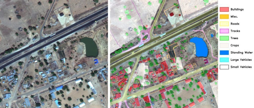
The challenge was organized by the Defence Science and Technology Laboratory (Dstl), an Executive Agency of the United Kingdom’s Ministry of Defence on Kaggle platform. As a training set, they provided 25 high-resolution satellite images representing 1 km² areas. The task was to locate 10 different types of objects:

1. Buildings
2. Miscellaneous manmade structures
3. Roads
4. Tracks
5. Trees
6. Crops
7. Waterway
8. Standing water
9. Large vehicles
10. Small vehicles

Sample image from the training set with labels.

These objects were not completely disjoint – you can find examples with vehicles on roads or trees within crops. The distribution of classes was uneven: from very common, such as crops (28% of the total area) and trees (10%), to much smaller such as roads (0.8%) or vehicles (0.02%). Moreover, most images only had a subset of classes.

Correctness of prediction was calculated using Intersection over Union (IoU, known also as Jaccard Index) between predictions and the ground truth. A score of 0 meant complete mismatch, whereas 1 – complete overlap. The score result was calculated for each class separately and then averaged. For our solution the average IoU was 0.46, whereas for the winning solution it was 0.49.

Preprocessing

For each image we were given three versions: grayscale, 3-band and 16-band. Details are presented in the table below:

Type	Wavebands	Pixel resolution	#channels	Size
grayscale	Panchromatic	0.31 m	1	3348 x 3392
3-band	RGB	0.31 m	3	3348 x 3392
16-band	Multispectral	1.24 m	8	837 x 848
	Short-wave infrared	7.5 m	8	134 x 136

We resized and aligned 16-band channels to match those from 3-band channels. Alignment was necessary to remove shifts between channels. Finally all channels were concatenated into single 20-channels input image.

Model

Our fully convolutional model was inspired by the family of U-Net architectures, where low-level feature maps are combined with higher-level ones, which enables precise localization. This type of network architecture was especially designed to effectively solve image segmentation problems. U-Net was the default choice for us and other competitors. If you would like more insights into architecture we suggest that you read the original paper. Our final architecture is depicted below:
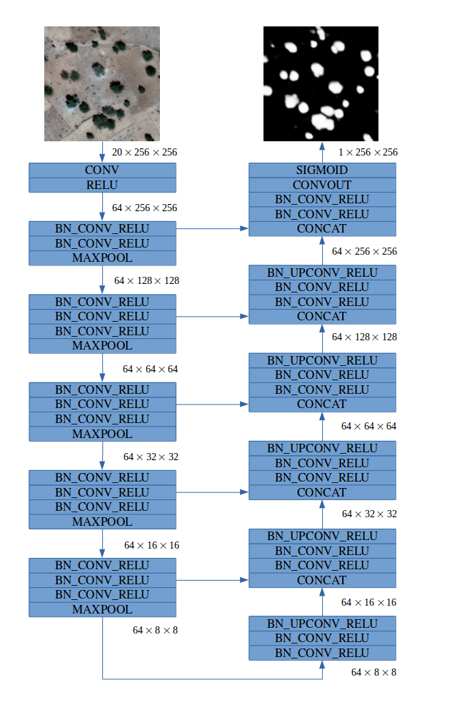For more details about specific modules click here.
Typical convolutional neural network (CNN) architecture involves increasing the number of feature maps (channels) with each max pooling operation. In our network we decided to keep a constant number of 64 feature maps throughout the network. This choice was motivated by two observations. Firstly, we can allow the network to lose some information after the downsampling layer because the model has access to low level features in the upsampling path. Secondly, in satellite images there is no concept of depth or high-level 3D objects to understand, so a large number of feature maps in higher layers may not be critical for good performance.
We developed separate models for each class, because it was easier to fine tune them individually for better performance and to overcome imbalanced data problems.

Training procedure

Models assign probability of belonging to a target class for each pixel from the input image. Although Jaccard was the evaluation metric, we used the per-pixel binary cross entropy objective for training.
We normalized images to have a zero mean and unit variance using precomputed statistics from the dataset. Depending on class we left preprocessed images unchanged or resized them together with corresponding label masks to 1024 x 1024 or 2048 x 2048 squares. During training we collected a batch of cropped 256 x 256 patches from different images where half of the images always contained some positive pixels (objects of target classes). We found this to be both the best and the simplest way to handle the imbalanced classes problem. Each image in a batch was augmented by randomly applying horizontal and vertical flips together with random rotation and color jittering.
Each model had approx. 1.7 million parameters. Its training (with batch size 4) from scratch took about two days on a single GTX 1070.

Predictions

We used a sliding window approach at test time with window size fixed to 256 x 256 and stride of 64. This allowed us to eliminate weaker predictions on image patch boundaries where objects may only be partially shown without context around them. To further improve prediction quality we averaged results for flipped and rotated versions of the input image, as well as for models trained on different scales. Overall we obtained well smoothed outputs.

Post-processing

Ground truth labels were provided in WKT format, presenting objects as polygons (defined by their vertices). It was necessary for us to generate submissions where polygons are concise and can be processed quickly by the evaluation system to avoid timeout limits. We found that this can be accomplished with minimal loss on the evaluation metric by using parameterized operations on binarized outputs. In our post-processing stage we used morphology dilation/erosion and simply removed objects/holes smaller than a given threshold.

Our solution

Buildings, Misc., Roads, Tracks, Trees, Crops, Standing Water

For these seven classes we were able to train convolutional networks (separately for each class) with binary cross entropy loss as described above on 20 channels inputs and two different scales (1024 and 2048) with satisfactory results. Outputs of the models were simply averaged and then post-processed with hyperparameters depending on particular classes.

Waterway

The solution for the waterway class was a combination of linear regression and random forest, trained on per pixel data from 20 input channels. Such a simple setup works surprisingly well because of the characteristic spectral response of water.

Large and Small Vehicles

We observed high variation of the results on the local validation and public leaderboard due to the small number of vehicles in the training set. To combat this we trained models separately for large and small vehicles, as well as single model for both of them (label masks were added together) on 20 channels inputs. Additionally, we repeated all experiments using 4 channels inputs (RGB + Panchromatic) to increase diversity of our models in ensemble. Outputs from models trained on both classes were averaged with single class specific models to produce final predictions for each type of vehicles.

Technologies

We implemented models in PyTorch and Keras (with TensorFlow backend), according to our team members’ preferences. Our strategy was to build separate models for each class, so this required careful management of our code. To run models and keep track of our experiments we used Neptune.

Final results

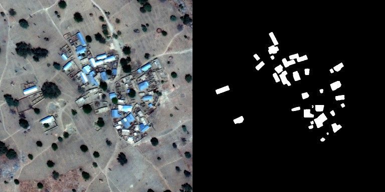
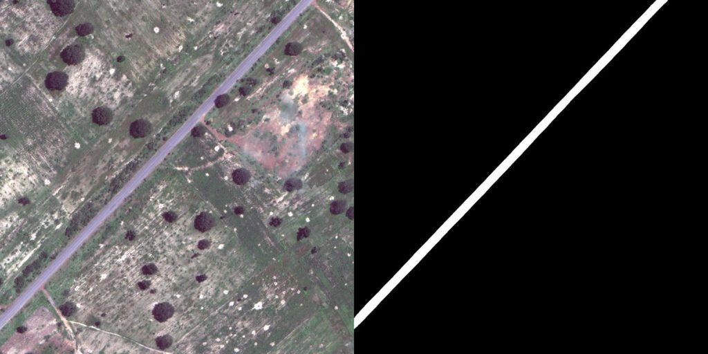
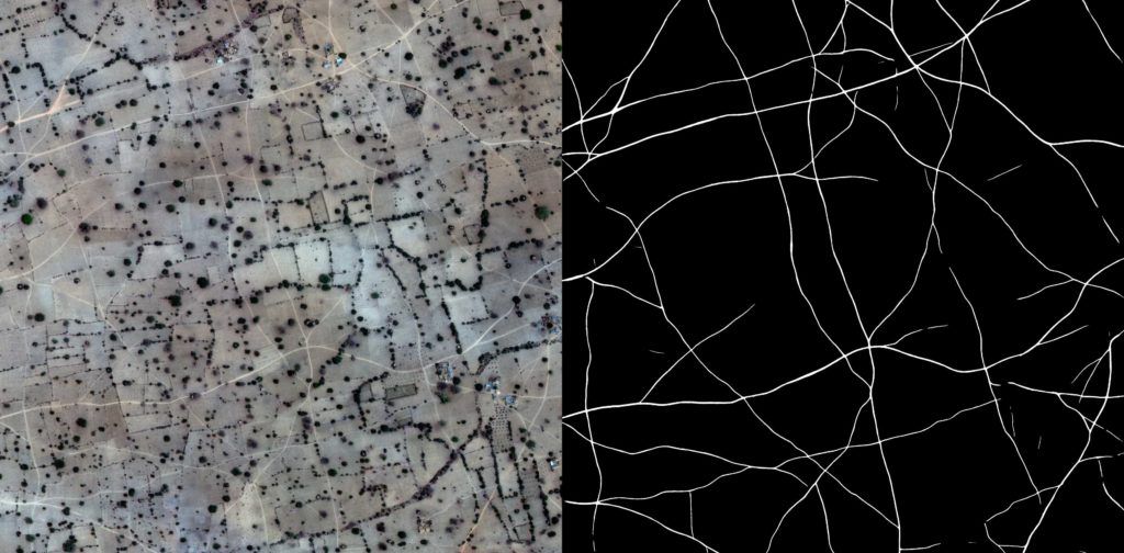
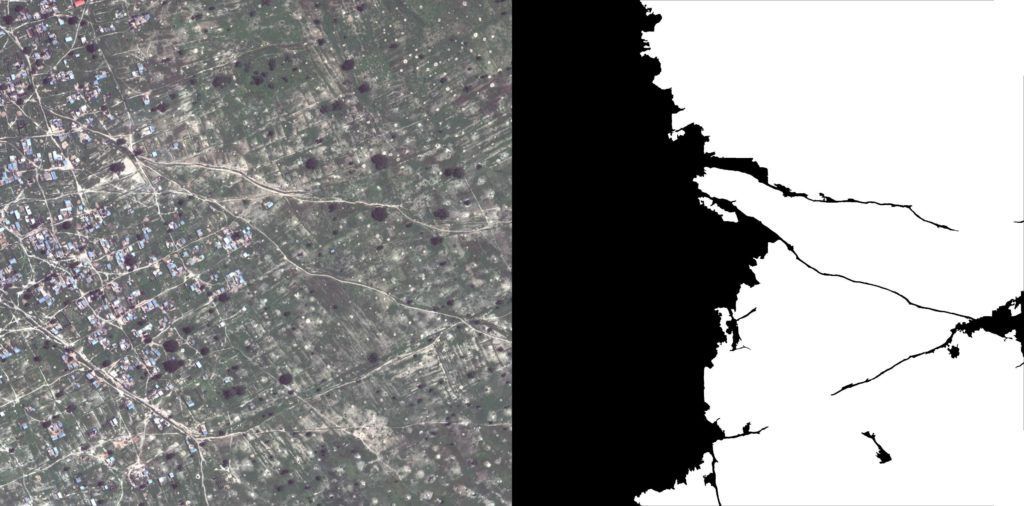
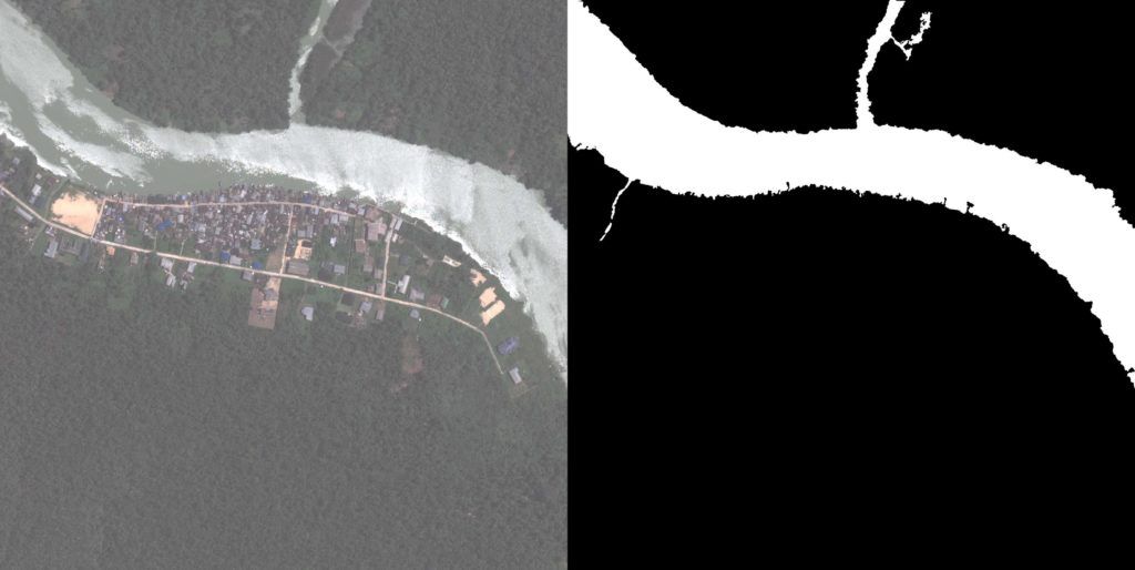
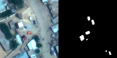
Below we present a small sample of the final results from our models:

Buildings

Roads

Tracks

Crops

Waterway

Small vehicles

Conclusions

Satellite imagery is a domain with a high volume of data which is perfect for deep learning. We have proved that the results gained from current state-of-the-art research can be applied to solve practical problems. Excited by our results, we look forward to more of such challenges in the future.
Team members:
Arkadiusz Nowaczyński
Michał Romaniuk
Adam Jakubowski
Michał Tadeusiak
Konrad Czechowski
Maksymilian Sokołowski
Kamil Kaczmarek
Piotr Migdał

Suggested readings

For those of you interested in additional reading, we recommend the following papers on image segmentation which inspired our work and success:

1. Fully Convolutional Networks for Semantic Segmentation
2. U-Net: Convolutional Networks for Biomedical Image Segmentation
3. The One Hundred Layers Tiramisu: Fully Convolutional DenseNets for Semantic Segmentation
4. Analyzing The Papers Behind Facebook’s Computer Vision Approach
5. Image-to-Image Translation with Conditional Adversarial Nets
6. ReSeg: A Recurrent Neural Network-based Model for Semantic Segmentation