
Training XGBoost with R and Neptune
In this blogpost we present the R library for Neptune – the DevOps platform for data scientists. Neptune’s R extension is presented by demonstrating the powerful XGBoost library and a bank marketing dataset (available at the UCI Machine Learning Repository).
The goal is to build a model that predicts how likely a given customer is to subscribe to a bank deposit. Such a model can be used as a basis for a recommendation system or for more efficient allocation of resources in a call center. The model is built by using XGBoost: a state-of-the-art library for training predictive models. XGBoost has a long legacy of successful applications in data science – here you can find a list of use cases in which it was used to win open machine learning challenges. If you are interested in more details and other modeling approaches to the problem under consideration we refer to this publication.
Let’s start with describing the dataset!
Bank customer data
The data we are dealing with here is a set of over 41K customer records from a bank. They comprise various features describing each customer. Among others, the provided data is the customer’s age, marital status and some other features regarding previous purchase history. We are also given a set of macroeconomic indicators, for example, the consumer confidence index. Finally, we are given the binary information whether a given customer subscribed for a bank deposit – about 11.3% of all customers decided to do so. Our goal is to build a model that gives the probability of this event.
Inquiries on subscribing to a bank deposit were made in a phone call. Along with data described above, we are also given information about how long such a call with each customer lasted. In the analysis, this feature should be disregarded as it would be considered a data leak. We want to train the model that gives information about the probability of subscribing to a deposit prior to taking any action (in particular, making a phone call). At the end of the day, we want to save resources and time spent on calling customers in vain.
We will employ relatively few preprocessing steps before plugging the data to the model. We will use the R’s model.matrix() function to encode categorical attributes. After this step, the data comprise 53 numeric attributes and a single target column. Loading the data and preprocessing is done using the code below. We also load all necessary libraries that we will use in this example: xgboost, neptune and ModelMetrics.
library(xgboost)
library(neptune)
library(ModelMetrics)
customer_data <- read.csv('https://s3-us-west-2.amazonaws.com/deepsense.neptune/data/bank-additional/bank-additional-full.csv', sep = ';')
customer_data$duration <- NULL
y <- customer_data$y == 'yes'
x <- model.matrix(y~.-1, data = customer_data)
Training XGBoost model
XGBoost is a powerful library for building ensemble machine learning models via the algorithm called gradient boosting. Training an XGBoost model is an iterative process. In each iteration, a new tree (or a forest) is built, which improves the accuracy of the current (ensemble) model.
In order to train and evaluate the model, we will split the data into three parts: a training set, a validation set and a test set. The training set will be used to build our model. With the validation set we will monitor the model’s performance on a different dataset than the training one. Finally, the test set will serve as a sanity check for the model’s final performance on a previously unseen holdout dataset. Here we decide to devote 60% of the data for training, 20% for validation and the remaining 20% for testing. For reproducibility we set a seed here.
set.seed(999)
train_valid_test <- sample(1:3, prob = c(0.6, 0.2, 0.2), replace = T, size = nrow(x))
train_idx <- train_valid_test == 1
valid_idx <- train_valid_test == 2
test_idx <- train_valid_test == 3
y_train <- y[train_idx]
y_valid <- y[valid_idx]
y_test <- y[test_idx]
x_train <- x[train_idx,]
x_valid <- x[valid_idx,]
x_test <- x[test_idx,]
At this point we should introduce an accuracy metric that we will employ. First, we note that there is some class imbalance in the response rate: as few as 1 out of 9 of all the responses are positive (this is typical in case of marketing data). In such applications, the area under the ROC curve (abbreviated as AUC) is often a metric of choice because it handles classification under imbalanced classes well. The rare class – customers subscribing to a deposit – is in this application of special interest for us.
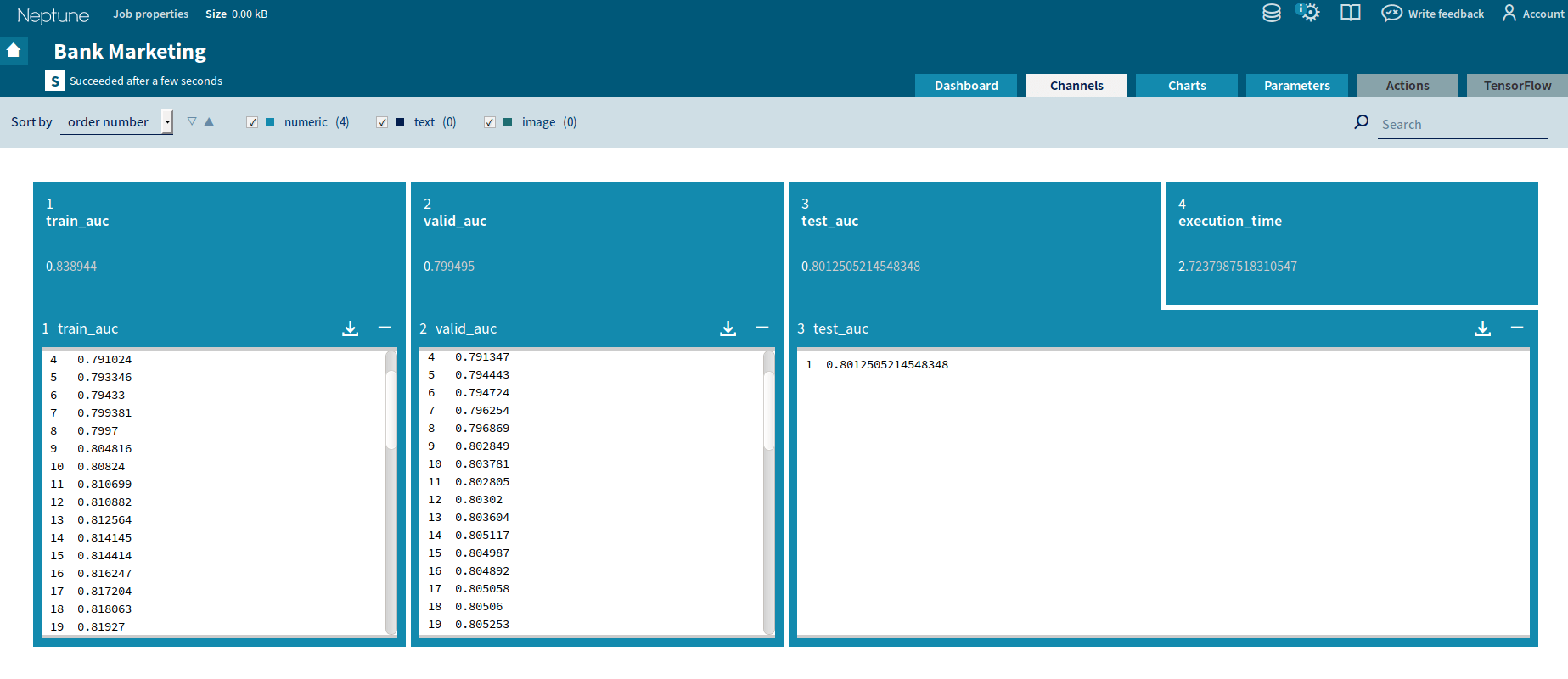
To monitor the training process in Neptune, we need to specify the appropriate Neptune channels. They are used for keeping track of metrics that are important to us. We will use two numeric channels – for the training and validation of the AUC scores. Finally, we are going to record the test AUC score. We can also keep track of other things like the training time for each iteration. On top of the channels we can create custom charts, which can be later viewed in Neptune’s Dashboard:
Below we set up the Neptune channels and Neptune charts:
createNumericChannel('train_auc')
createNumericChannel('valid_auc')
createNumericChannel('test_auc')
createChart(chartName = 'Train & validation auc', series = list('train_auc', 'valid_auc'))
createNumericChannel('execution_time')
createChart(chartName = 'Total execution time', series = list('execution_time'))
Neptune facilitates monitoring our computations that are organized in a process called a job. When executing the job, created channels will be visible for inspection in Neptune’s menu. So far we defined four numeric channels and two charts. After executing the job, you can view the channels in Neptune’s UI:
Yet another useful feature of XGBoost is the possibility of calling a custom callback function after each iteration of the boosting algorithm. Callbacks are useful functions for debugging and online performance monitoring of your models. We will write our own function to keep track of the training process. Here you can see some examples of callback functions. We will specifically overwrite the function cb.print.evaluation() from the repository so that we can track the progress of learning in Neptune. This function is presented below. The variable start_time is a global variable that allows us to monitor the total execution time (we will create it in the next step).
cb.print.evaluation <- function (period = 1) {
  callback <- function(env = parent.frame()) {
    if (length(env$bst_evaluation) == 0 || period == 0)
      return()
    i <- env$iteration
    if ((i - 1)%%period == 0 || i == env$begin_iteration || i == env$end_iteration) {
      channelSend('train_auc', i, env$bst_evaluation[1])
      channelSend('valid_auc', i, env$bst_evaluation[2])
      channelSend('execution_time', i, as.numeric(Sys.time() - start_time))
    }
  }
  attr(callback, 'call') <- match.call()
  attr(callback, 'name') <- 'cb.print.evaluation'
  callback
}
Note that the function refers to its parent environment that it is called from – the parent.frame() function. This allows us to access the objects created during the training process (in this case we choose to monitor both the training and validation of the AUC scores). We can access them all by referring to the parent environment as shown above.
The conditional instructions in the code above check if any monitoring was set and then performs it in every period of iterations (this can be changed via the parameter print.every.n in the xgb.train() function), for the first and last iteration.
Next, we train our model. To start, we create a start_time variable to monitor the execution time.
start_time <- Sys.time()
model <- xgb.train(
params = list(
objective = 'binary:logistic',
eval_metric = 'auc',
max_depth = 4),
data = xgb.DMatrix(x_train, label = y_train),
nrounds = 50,
watchlist = list(
  train = xgb.DMatrix(x_train, label = y_train),
  validation = xgb.DMatrix(x_valid, label = y_valid)),
  callbacks = list(cb.print.evaluation()))
Let’s have a closer look at what is going on here. Above, the training and validation sets for performance monitoring are submitted to the model as the parameter named watchlist. Some extra configuration needs to be done. We set:
- evaluation metric to be AUC (parameter eval_metric = ‘auc’)
- learning task as a binary classification with logistic loss (objective = ‘binary:logistic’)
- maximal depth of individual tree depth to 4 – an arbitrary value (max_depth = 4)
- number of boosting iterations to 50 (nrounds = 50).
To finalize the preparations we need to specify a configuration file for Neptune with some metadata. For now it may be as simple as the exemplary file below.
name: Bank Marketing
project: Predicting Deposit Subscription
We can run our code with Neptune in command line with:
$neptune run bank_marketing.R --config xgb_config.yaml --dump-dir-url my_dump_dir
The file bank_marketing.R is our model’s R code. The file name xgb_config.yaml represents Neptune’s configuration and the dump_dir is a directory where all the job’s output and source code will be stored. This is useful for the reproducibility of the experiment.
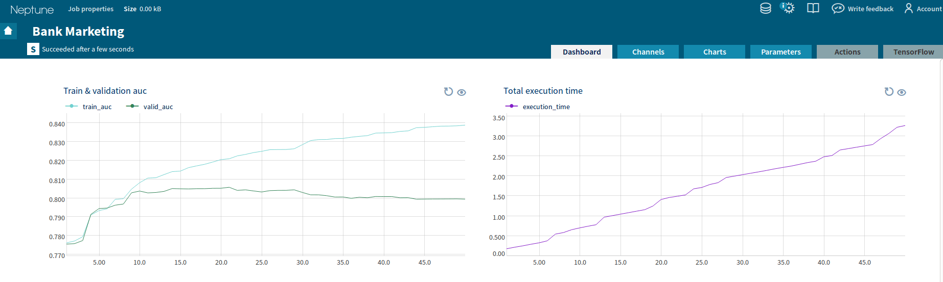
In Neptune’s dashboard we can see both the training and validation of the AUC scores on a plot.

XGBoost has a useful parameter early_stopping. This parameter stops further training, when the evaluation metric values for the validation set does not improve for the next early_stopping iterations. In machine learning, it is a common way to prevent the overfitting of a model. However, it is not known in advance to what value you have to set this parameter to. The idea here is to plot the training and validation of loss and observe the moment when the training is no longer necessary. From the visualization of the training process above it appears that 10 is a sufficient number of iterations (trees) in our ensemble model. In this way, we also arrive at a less complex model with no loss of its accuracy.
We also changed the random seed above to observe if we arrive at a stable solution for different data shuffles (see train/validation/test split above). In general, based on our experimentation, the ensemble of 10 trees (that is, running the model for 10 iterations) appears to produce a decent and stable model overall. Here, Neptune helps us diagnose a proper early stopping time via presentation of accuracy scores. Finally, it is convenient to set the number of iterations as the job parameter and extend the configuration file as discussed here. For example, in Neptune’s R library, the command line argument nrounds can be accessed in the job via the nrounds <- params(‘nrounds’) command.
It’s time to inspect the model performance on the reminder set of records.
Model evaluation and the lift curve
Finally, we make predictions and evaluate the model using the holdout test set. Using parameter ntreelimit we may specify the model built after 10 iterations to be used for predicting new data (as discussed above).
predictions_test <- predict(model, xgb.DMatrix(x_test), ntreelimit = 10)
auc_test <- auc(y_test, predictions_test)
Evaluation yields 0.80 AUC. This score is close to the accuracy obtained on the validation set, which is good: we created a stable model with no sign of overfitting – it is ready to be used!
Let’s apply it to the holdout test set and measure its effectiveness on the lift chart. This is a tool for getting insight into the expected performance of our marketing campaign if we target it for the most likely customers as predicted by the model.
To produce the lift chart, we sort the true responses (y_test) according to the probability of deposit subscription in a decreasing order and compute a cumulative fraction of responses. This fraction is also normalized against the baseline level equal to the fraction of responses in the test data (11.7%). We create an extra numeric channel and a chart for the lift curve and plot it for top 10%, 20%, …., 100% of customers. This is accomplished using the function below.
lift_chart <- function(responses, predictions) {
  baseline <- mean(responses)
  responses_ordered <- responses[order(predictions, decreasing = TRUE)]
  lift <- cumsum(responses_ordered) / 1:length(responses_ordered) / baseline
  createNumericChannel('lift')
  createChart(chartName = 'Lift chart', series = list('lift'))
  n <- length(lift)
  for(x in seq(0.1, 1, by = 0.1)) {
    # max(., 1) assures a proper index >= 1
    channelSend('lift', x, lift[max(round(x * n), 1)])
  }
}
lift_chart(y_test, predictions_test)
In Neptune’s dashboard this produces an interactive plot named “Lift chart” presented below.
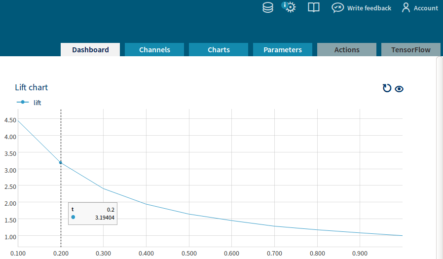
Based on this chart, we may analyze our results in greater detail. For example, we see that contacting top 20% of customers (as selected by our model) translates to over 3-fold increase in the hit rate (that is, the fraction of subscriptions in the selected group) as compared to the baseline level for the test data. This results in a more efficient targeting of our campaign. In practice, the desired number of contacted customers depends on the resources available and costs associated with contacting them.
The end
That’s all! We trained a model to predict how likely a customer is to order a given bank product. Using R and XGBoost with the help of Neptune, we trained a model and tracked its learning process. There is still room for improvement of the accuracy of the model. Playing with the parameters described above would be a good starting point here. You can give it a try and access the complete workflow at our Github repository (for the 1.4 version) or explore the job in NeptuneGo!.
This is our first attempt at integrating Neptune with R. We will be very grateful for your feedback here! We would like to make sure that it fits well with your experimentation pipeline. Moreover, we hope that it can improve your pipeline as dramatically as Neptune’s Python API changed our experience.