Using deep learning for Single Image Super Resolution
Single Image Super Resolution involves increasing the size of a small image while keeping the attendant drop in quality to a minimum. The task has numerous applications, including in satellite and aerial imaging analysis, medical image processing, compressed image/video enhancement and many more. In this blog post we apply three deep learning models to this problem and discuss their limitations and promising ways to overcome them.
Single Image Super Resolution: Problem statement
Our objective is to take a low resolution image and produce an estimate of a corresponding high‑resolution image. This problem is ill‑posed – multiple high‑resolution images can be produced from the same low‑resolution image. For instance, suppose we have a 2×2 pixel sub‑image containing a small vertical or horizontal bar [Fig. 1]. Regardless of the orientation of the bar, these 4 pixels will correspond to just one pixel in a picture downscaled 4 times. With real life images, one needs to overcome an abundance of similar problems, making the task difficult to solve.

prediction of a model trained to minimize MSE loss
First, let’s introduce a quantitative quality‑measurement method to evaluate and compare the models. For each model implemented, we will compute a metric commonly used to measure the quality of reconstruction of lossy compression codecs, called Peak Signal to Noise Ratio (PSNR). This metric is a de‑facto standard used in Super Resolution research. It measures how much the distorted image (possibly of lower quality) deviates from the original high‑quality image. In this setting, PSNR is the ratio of maximum possible pixel value of the image (signal strength) to maximum mean squared error (MSE) between the original image and its estimated version (noise strength), expressed in logarithmic scale.
\(PSNR = 10 cdot log_{10}frac{MAX_I^2}{MSE}\)
The larger the PSNR values, the better the reconstruction, and therefore maximization of PSNR naturally leads to minimizing MSE as the objective function. That was our approach in two out of three models we present here.
In our experiments, we trained the models to upscale input images four times (in terms of width and height). Above this factor, upscaling even small images becomes hard – for example, an image upscaled eight times has a 64x bigger pixel count. Storing it consequently requires 64x more memory in raw form, to which it is converted during training.
We have tested our models on benchmarks commonly used in the literature – Set5, Set14 and BSD100. The performance of the models described on these datasets is cited in the papers, which allowed us to compare our results to those other authors have put forward.
The models were implemented in PyTorch, an open‑source neural network framework developed by Facebook.
Why deep learning?
One of the most commonly used techniques for upscaling an image is interpolation. Although simple to implement, this method leaves much to be desired in terms of visual quality, as the details (e.g. sharp edges) are often not preserved.


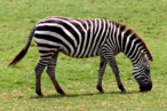
nearest neighbour interpolation, bilinear interpolation and bicubic interpolation. The image
was upscaled 4x.
More sophisticated methods exploit internal similarities of a given image or use datasets of low‑resolution images and their high‑resolution counterparts, effectively learning a mapping between them. Among example‑based SR algorithms, the sparse‑coding‑based method is one of the most popular.
This method requires a dictionary to be found that will allow us to map low resolution images into an intermediate, sparse representation. In addition, the HR dictionary is learned, and will allow us to restore our estimate of a high resolution image. Such a pipeline usually involves several steps and not all of them can be optimized. Ideally we would like to have all of these steps combined in one big step with all of its parts being optimizable. That effect can be achieved by a neural network, the architecture of which is inspired by sparse coding.
See more here.
SRCNN
SRCNN was the first deep learning method to outperform traditional ones. It is a convolutional neural network consisting of only 3 convolutional layers: patch extraction and representation, non‑linear mapping and reconstruction.
Before being fed into the network, an image needs to be upsampled via bicubic interpolation. It’s then converted to YCbCr color space, while only luminance channel (Y) is used by the network. The network’s output is then merged with interpolated CbCr channels to produce a final color image. We chose this procedure because we are not interested in changing colors (this is the information stored in the CbCr channels), but only their brightness (the Y channel), and ultimately because human vision is more sensitive to luminance (“black and white”) differences than chromatic differences.
We found SRCNN really difficult to train. It was sensitive to hyperparameter changes, and the set‑up presented in the paper (learning rate 10-4 for the first two layers, 10-5 for the last layer, SGD optimizer) caused our PyTorch implementation to produce sub‑optimal results. We observed small changes under some different learning rates, but in the end the thing that gave us the biggest performance boost was switching to Adam optimizer, with a learning rate of 10-5 used for all layers. The final network was trained on 14k 32×32 subimages from the same dataset as in original paper (91 images).

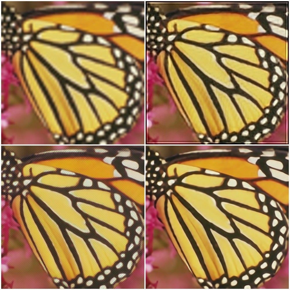
perceptual loss and SRResNet images were produced by our implementations of corresponding models.
Perceptual loss
Although SRCNN is already better than standard methods, there are some ways in which it can still be enhanced. As mentioned earlier, the network is unstable, and one may also wonder whether optimizing MSE is an optimal choice.
Clearly, the images obtained by minimizing MSE are overly smooth. (MSE tends to produce an image resembling the mean of all possible high resolution pictures, resulting in a given low resolution picture [Fig. 1]). MSE also does not capture the perceptual differences between the model’s output and the ground truth image. Consider a pair of images, where the second one is a copy of the first, but shifted a few pixels to the left. For a human the copy looks almost indistinguishable from the original, but even such a small change can cause PSNR to decrease dramatically.
How should the perceived content of a given image be preserved? A similar arises in neural style transfer, and perceptual loss is a potential solution. It too optimizes MSE, but instead of using the model output itself, one can use the high‑level image feature representations extracted from pretrained convolutional neural networks (in our case output from 7th layer of VGG16). The intuition behind this idea is that a network trained for image classification (like VGG) stores in its feature maps the information on what details of common objects look like. And we want our upscaled image to be made up of objects resembling real world ones as much as possible.
Apart from changing the loss function, network architecture is also remodeled. The model is much deeper than SRCNN, uses residual blocks and does most of the processing on low‑resolution images (which accelerates training and inference). Upscaling also happens inside the network. In their paper, the authors used transposed convolutions (also called deconvolutions) with kernel 3×3 and stride=2 for that purpose. Artifacts produced by this model seemed similar to those known as the checkerboard effect. To reduce this effect we also tried deconvolution with a 4×4 kernel and nearest neighbor interpolation followed by a 3×3 convolutional layer with stride=1. In the end, interpolation followed by convolutional layer gave the best results, but didn’t remove the artifacts completely. Similar effects were observed in the original report.
Similar to the process described in paper, our training pipeline consisted of a dataset of 288×288 random crops from nearly 10k images from MS‑COCO. We set the learning rate to 10-3 and used Adam as our optimizer. Unlike in the paper cited above, we skipped post‑processing (histogram matching) as it didn’t provide any improvement.
SRResNet
In order to maximise our PSNR performance, we decided to implement a network called SRResNet, which achieves state‑of‑the‑art results on standard benchmarks. The original paper mentions a way of extending it in a way that allows more high frequency details to be restored.
As with the residual network described in the previous paragraph, SRResNet’s residual blocks architecture is based on this post. There are two minor additions: first, SRResNet uses Parametric ReLU instead of ReLU, which generalizes the former by introducing a learnable parameter that makes it possible to adaptively learn the negative part coefficient. The other difference is the image upsampling method used – in SRResNet, sub‑pixel convolutional layers are used. This technique is thoroughly explained here.
The images generated by the SRResNet we trained are almost indistinguishable from the results presented in the paper. The training took two days, during which we used Adam optimizer with a learning rate of 10-4. The dataset used consisted of 96×96 random crops from MS‑COCO, similar to the perceptual loss network.
Future work
There are several promising deep learning‑based approaches to single image super resolution that we didn’t test due to time constraints.
This recent paper mentions superb PSNR results gained thanks to the use of a modified SRResNet architecture. The authors remove batch normalization from the residual layers, and increase the number of residual layers used from 16 to 32. The resulting network trains for seven days on NVIDIA Titan Xs. Our implementation of SRResNet trained for two days to get our results, which allowed for faster iterations and more efficient hyperparameter tuning, but would not be possible had the ideas described been implemented.
Our perceptual loss experiments show that PSNR may not be a good metric to use for evaluating super resolution networks. In our opinion, more research needs to be done on different types of perceptual loss. In the papers we have examined, we’ve only seen simple MSE between VGG feature map representations of network output and ground truth. It’s unclear why MSE, being a per‑pixel loss, would be a good choice in this case.
Another promising direction for super resolution is Generative Adversarial Networks. This original paper extends SRResNet by using it as part of the architecture called SRGAN. Images generated by the resulting network contain high frequency details, like animals’ fur or grass straws. While they may look more believable, the images generated suffer in the PSNR statistics.


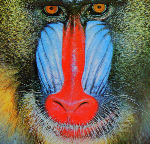
the image produced by SRResNet extension, and the original image
Conclusion
In this blogpost we have described our experiments with three different convolutional neural networks used for Single Image Super Resolution. The table below summarizes our results.
| SRCNN | Perceptual loss | SRResNet |
| + short inference + better than standard methods – worst results among deep learning approaches |
+ more natural looking results than SRCNN – strong artifacts |
+ state‑of‑the‑art results – long inference |
Even a simple three layer SRCNN was able to beat most non‑deep‑learning methods when measured on standard benchmark datasets using PSNR. Our examinations of perceptual loss showed, however, that this measure is not perfect for evaluating our model’s performance, as we were able to produce visually appealing images that were much worse than bicubic interpolation when evaluated with PSNR. Finally, we reimplemented SRResNet and reproduced state‑of‑the‑art results on benchmark datasets.
References
[1] Image Super‑Resolution Using Deep Convolutional Networks
[2] Perceptual Losses for Real‑Time Style Transfer and Super‑Resolution
[3] Photo‑Realistic Single Image Super‑Resolution Using a Generative Adversarial Network
[4] Enhanced Deep Residual Networks for Single Image Super‑Resolution
[5] Real‑Time Single Image and Video Super‑Resolution Using an Efficient Sub‑Pixel Convolutional Neural Network
[6] Training and investigating Residual Nets


