Between now and the end of 2017, deepsense.ai will run 30 machine learning and deep learning seminars at prestigious universities across Europe as part of the effort to scale the Intel® Nervana™ AI Academy for students in EMEA.
deepsense.ai will train hundreds of European students in the upcoming three months as part of the Intel® Nervana™ AI Academy. Students will get the valuable opportunity to gain practical knowledge in two of the most cutting‑edge and fast developing areas of data science, machine learning and deep learning.
deepsense.ai organizes seminars and delivers machine learning and deep learning sessions, giving students a great chance to meet professional data science practitioners and ask them even the most challenging questions on advanced analytics. At the seminars, participants are also encouraged to join Intel’s Student Ambassador Program and work on their machine learning projects with infrastructural and financial support from Intel.
deepsense.ai CEO Tomasz Kułakowski stressed the importance of the collaboration with Intel: “I’m glad that deepsense.ai’s artificial intelligence expertise has been recognized by Intel and our company has been invited to support the Intel Nervana AI Academy in EMEA – that’s a project with great potential to successfully promote the most innovative approaches to data analytics today and grow new generations of talented data scientists from the leading academic communities. It requires time and full determination to build data science competencies at the highest level of excellence. deepsense.ai offers professional technical and business workshops as a part of our comprehensive approach to our clients’ needs – we’re open to sharing our know‑how with any company eager to upskill in AI.”
deepsense.ai shares Intel’ vision for making artificial intelligence solutions more approachable and widely used in daily life. To that end: deepsense.ai delivers break‑through end‑to‑end data science solutions while Intel builds the powerful hardware needed to process data effectively. Their experience in data science has allowed each of them also to create dedicated tools for data scientists, deepsense.ai Neptune and Intel® Nervana.
###
About deepsense.ai:
Media contact:
deepsense.ai trademarks at boilerplate
https://deepsense.ai/wp-content/uploads/2019/02/deepsense-ai-popularize-machine-learning-at-european-universities-as-part-of-the-intel-nervana-ai-academy.jpg3371140Barbara Rutkowskahttps://deepsense.ai/wp-content/uploads/2023/10/Logo_black_blue_CLEAN_rgb.pngBarbara Rutkowska2017-10-24 12:39:032023-07-16 19:27:23deepsense.ai popularizes machine learning at European universities as part of the Intel Nervana AI Academy
At deepsense.ai, we’re doing our best to make our mark in state‑of‑the‑art data science. For many years, we have been competing in machine learning challenges, gaining both conceptual and technical expertise. Now, we have decided to open source an end‑to‑end image classification sample solution for the ongoing Cdiscount Kaggle competition. In so doing, we believe we’ll encourage data scientists both seasoned and new to compete on Kaggle and test their neural nets.
Introduction
Competing in machine learning challenges is fun, but also a lot of work. Participants must design and implement end‑to‑end solutions, test neural architectures and run dozens of experiments to train deep models properly. But this is only a small part of the story. Strong Kaggle competition solutions have advanced data pre‑ and post‑processing, ensembling and validation routines, to name just a few. At this point, competing effectively becomes really complex and difficult to manage, which may discourage some data scientists from rolling up their sleeves and jumping in. Here at deepsense.ai we believe that Kaggle is a great platform for advanced data scientific training at any level of expertise. So great, in fact, that we felt compelled to open‑source an image classification sample solution to the currently open Cdiscount challenge. Below, we describe what we have prepared.
When we say our solution is end‑to‑end, we mean that we started with raw input data downloaded directly from the Kaggle site (in the bson format) and finish with a ready‑to‑upload submit file. Here are the components:
data loader
Keras custom iterator for bson file
label encoder representing product IDs to fit the Keras API
neural network training on n classes and k examples per class. We use the following architectures:
You are encouraged to replace our network with your own. Below you can find a short snippet of code that you simply place in the models.py file:
class MyModel(BasicKerasClassifier):
    def _build_model(self, params):
        return Model
Otherwise I would suggest extending BasicKerasClassifier, or KerasDataLoader with custom augmentations, learning rate schedules and other tricks of your choice.
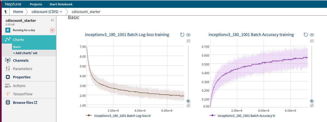
Feel free to use, modify and run this code for your own purposes. We run multiple of them on Neptune, which you may find useful for managing your experiments.
Single Image Super Resolution involves increasing the size of a small image while keeping the attendant drop in quality to a minimum. The task has numerous applications, including in satellite and aerial imaging analysis, medical image processing, compressed image/video enhancement and many more. In this blog post we apply three deep learning models to this problem and discuss their limitations and promising ways to overcome them.
Single Image Super Resolution: Problem statement
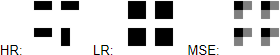
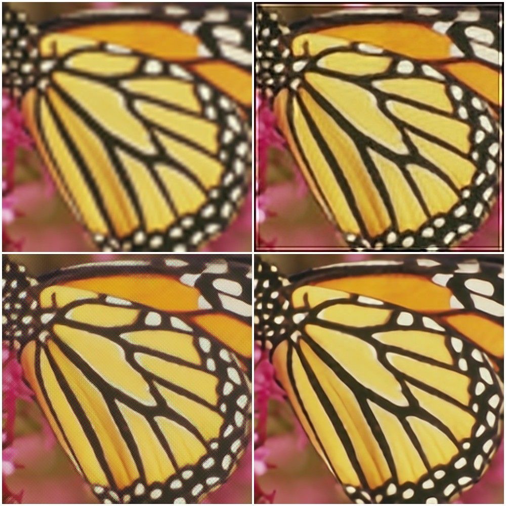
Our objective is to take a low resolution image and produce an estimate of a corresponding high‑resolution image. This problem is ill‑posed – multiple high‑resolution images can be produced from the same low‑resolution image. For instance, suppose we have a 2×2 pixel sub‑image containing a small vertical or horizontal bar [Fig. 1]. Regardless of the orientation of the bar, these 4 pixels will correspond to just one pixel in a picture downscaled 4 times. With real life images, one needs to overcome an abundance of similar problems, making the task difficult to solve.
Figure 1: from left to right, ground truth HR image, corresponding LR image,
prediction of a model trained to minimize MSE loss
First, let’s introduce a quantitative quality‑measurement method to evaluate and compare the models. For each model implemented, we will compute a metric commonly used to measure the quality of reconstruction of lossy compression codecs, called Peak Signal to Noise Ratio (PSNR). This metric is a de‑facto standard used in Super Resolution research. It measures how much the distorted image (possibly of lower quality) deviates from the original high‑quality image. In this setting, PSNR is the ratio of maximum possible pixel value of the image (signal strength) to maximum mean squared error (MSE) between the original image and its estimated version (noise strength), expressed in logarithmic scale.
\(PSNR = 10 cdot log_{10}frac{MAX_I^2}{MSE}\)
The larger the PSNR values, the better the reconstruction, and therefore maximization of PSNR naturally leads to minimizing MSE as the objective function. That was our approach in two out of three models we present here.
In our experiments, we trained the models to upscale input images four times (in terms of width and height). Above this factor, upscaling even small images becomes hard – for example, an image upscaled eight times has a 64x bigger pixel count. Storing it consequently requires 64x more memory in raw form, to which it is converted during training.
We have tested our models on benchmarks commonly used in the literature – Set5, Set14 and BSD100. The performance of the models described on these datasets is cited in the papers, which allowed us to compare our results to those other authors have put forward.
The models were implemented in PyTorch, an open‑source neural network framework developed by Facebook.
One of the most commonly used techniques for upscaling an image is interpolation. Although simple to implement, this method leaves much to be desired in terms of visual quality, as the details (e.g. sharp edges) are often not preserved.
Figure 2: Most common interpolation methods produce blurry images. From top to bottom:
nearest neighbour interpolation, bilinear interpolation and bicubic interpolation. The image
was upscaled 4x.
More sophisticated methods exploit internal similarities of a given image or use datasets of low‑resolution images and their high‑resolution counterparts, effectively learning a mapping between them. Among example‑based SR algorithms, the sparse‑coding‑based method is one of the most popular.
This method requires a dictionary to be found that will allow us to map low resolution images into an intermediate, sparse representation. In addition, the HR dictionary is learned, and will allow us to restore our estimate of a high resolution image. Such a pipeline usually involves several steps and not all of them can be optimized. Ideally we would like to have all of these steps combined in one big step with all of its parts being optimizable. That effect can be achieved by a neural network, the architecture of which is inspired by sparse coding.
See more here.
SRCNN
SRCNN was the first deep learning method to outperform traditional ones. It is a convolutional neural network consisting of only 3 convolutional layers: patch extraction and representation, non‑linear mapping and reconstruction.
Before being fed into the network, an image needs to be upsampled via bicubic interpolation. It’s then converted to YCbCr color space, while only luminance channel (Y) is used by the network. The network’s output is then merged with interpolated CbCr channels to produce a final color image. We chose this procedure because we are not interested in changing colors (this is the information stored in the CbCr channels), but only their brightness (the Y channel), and ultimately because human vision is more sensitive to luminance (“black and white”) differences than chromatic differences.
We found SRCNN really difficult to train. It was sensitive to hyperparameter changes, and the set‑up presented in the paper (learning rate 10-4 for the first two layers, 10-5 for the last layer, SGD optimizer) caused our PyTorch implementation to produce sub‑optimal results. We observed small changes under some different learning rates, but in the end the thing that gave us the biggest performance boost was switching to Adam optimizer, with a learning rate of 10-5 used for all layers. The final network was trained on 14k 32×32 subimages from the same dataset as in original paper (91 images).
Figure 3: Upper left – bicubic interpolation, upper right – SRCNN, bottom left – perceptual loss, bottom right – SRResNet. SRCNN,
perceptual loss and SRResNet images were produced by our implementations of corresponding models.
Perceptual loss
Although SRCNN is already better than standard methods, there are some ways in which it can still be enhanced. As mentioned earlier, the network is unstable, and one may also wonder whether optimizing MSE is an optimal choice.
Clearly, the images obtained by minimizing MSE are overly smooth. (MSE tends to produce an image resembling the mean of all possible high resolution pictures, resulting in a given low resolution picture [Fig. 1]). MSE also does not capture the perceptual differences between the model’s output and the ground truth image. Consider a pair of images, where the second one is a copy of the first, but shifted a few pixels to the left. For a human the copy looks almost indistinguishable from the original, but even such a small change can cause PSNR to decrease dramatically.
How should the perceived content of a given image be preserved? A similar arises in neural style transfer, and perceptual loss is a potential solution. It too optimizes MSE, but instead of using the model output itself, one can use the high‑level image feature representations extracted from pretrained convolutional neural networks (in our case output from 7th layer of VGG16). The intuition behind this idea is that a network trained for image classification (like VGG) stores in its feature maps the information on what details of common objects look like. And we want our upscaled image to be made up of objects resembling real world ones as much as possible.
Apart from changing the loss function, network architecture is also remodeled. The model is much deeper than SRCNN, uses residual blocks and does most of the processing on low‑resolution images (which accelerates training and inference). Upscaling also happens inside the network. In their paper, the authors used transposed convolutions (also called deconvolutions) with kernel 3×3 and stride=2 for that purpose. Artifacts produced by this model seemed similar to those known as the checkerboard effect. To reduce this effect we also tried deconvolution with a 4×4 kernel and nearest neighbor interpolation followed by a 3×3 convolutional layer with stride=1. In the end, interpolation followed by convolutional layer gave the best results, but didn’t remove the artifacts completely. Similar effects were observed in the original report.
Similar to the process described in paper, our training pipeline consisted of a dataset of 288×288 random crops from nearly 10k images from MS‑COCO. We set the learning rate to 10-3 and used Adam as our optimizer. Unlike in the paper cited above, we skipped post‑processing (histogram matching) as it didn’t provide any improvement.
In order to maximise our PSNR performance, we decided to implement a network called SRResNet, which achieves state‑of‑the‑art results on standard benchmarks. The original paper mentions a way of extending it in a way that allows more high frequency details to be restored.
As with the residual network described in the previous paragraph, SRResNet’s residual blocks architecture is based on this post. There are two minor additions: first, SRResNet uses Parametric ReLU instead of ReLU, which generalizes the former by introducing a learnable parameter that makes it possible to adaptively learn the negative part coefficient. The other difference is the image upsampling method used – in SRResNet, sub‑pixel convolutional layers are used. This technique is thoroughly explained here.
The images generated by the SRResNet we trained are almost indistinguishable from the results presented in the paper. The training took two days, during which we used Adam optimizer with a learning rate of 10-4. The dataset used consisted of 96×96 random crops from MS‑COCO, similar to the perceptual loss network.
Future work
There are several promising deep learning‑based approaches to single image super resolution that we didn’t test due to time constraints.
This recent paper mentions superb PSNR results gained thanks to the use of a modified SRResNet architecture. The authors remove batch normalization from the residual layers, and increase the number of residual layers used from 16 to 32. The resulting network trains for seven days on NVIDIA Titan Xs. Our implementation of SRResNet trained for two days to get our results, which allowed for faster iterations and more efficient hyperparameter tuning, but would not be possible had the ideas described been implemented.
Our perceptual loss experiments show that PSNR may not be a good metric to use for evaluating super resolution networks. In our opinion, more research needs to be done on different types of perceptual loss. In the papers we have examined, we’ve only seen simple MSE between VGG feature map representations of network output and ground truth. It’s unclear why MSE, being a per‑pixel loss, would be a good choice in this case.
Another promising direction for super resolution is Generative Adversarial Networks. This original paper extends SRResNet by using it as part of the architecture called SRGAN. Images generated by the resulting network contain high frequency details, like animals’ fur or grass straws. While they may look more believable, the images generated suffer in the PSNR statistics.
Figure 4: From top to bottom: the image produced by our SRResNet implementation,
the image produced by SRResNet extension, and the original image
In this blogpost we have described our experiments with three different convolutional neural networks used for Single Image Super Resolution. The table below summarizes our results.
SRCNN
Perceptual loss
SRResNet
+ short inference
+ better than standard methods
– worst results among deep learning approaches
+ more natural looking results than SRCNN
– strong artifacts
+ state‑of‑the‑art results
– long inference
Figure 5: Advantages and disadvantages of the models discussed
Even a simple three layer SRCNN was able to beat most non‑deep‑learning methods when measured on standard benchmark datasets using PSNR. Our examinations of perceptual loss showed, however, that this measure is not perfect for evaluating our model’s performance, as we were able to produce visually appealing images that were much worse than bicubic interpolation when evaluated with PSNR. Finally, we reimplemented SRResNet and reproduced state‑of‑the‑art results on benchmark datasets.
https://deepsense.ai/wp-content/uploads/2019/02/using-deep-learning-for-single-image-super-resolution.jpeg3371140Katarzyna Kańskahttps://deepsense.ai/wp-content/uploads/2023/10/Logo_black_blue_CLEAN_rgb.pngKatarzyna Kańska2017-10-23 09:17:272024-03-11 15:45:24Using deep learning for Single Image Super Resolution
We’re thrilled today to announce the latest version of Neptune: Machine Learning Lab. This release will allow data scientists using Neptune to take some giant steps forward. Here we take a quick look at each of them.
Cloud support
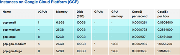
One of the biggest differences between Neptune 1.x and 2.x is that 2.x supports Google Cloud Platform. If you want to use NVIDIA® Tesla® K80 GPUs to train your deep learning models or Google’s infrastructure for your computations, you can just select your machine type and easily send your computations to the cloud. Of course, you can still run experiments on your hardware the way it was. We currently support only GCP–but stay tuned as we will not only be bringing more clouds and GPUs into the Neptune support fold, but offering them at even better prices!
With cloud support, we are also changing our approach to managing data. Neptune uses shared storage to store data about each experiment, for both the source code and the results (channel values, logs, output files, e.g. trained models). On top of that, you can upload any data to a project and use it in your experiments. As you execute your experiments, you’ve got all your sources at your fingertips, in the /neptune directory, which is available on fast drive for reading and writing. It is also your current working directory – just like you would run it on your local machine. Alongside this feature, Neptune can still keep your original sources so you can easily reproduce your experiments. For more details please read documentation.
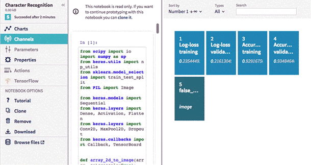
Interactive Notebooks
Engineers love how interactive and easy to use Notebooks are, so it should come as no surprise that they’re among the most frequently used data science tools. Neptune now allows you to prototype faster and more easily using Jupyter Notebooks in the cloud, which is fully integrated with Neptune. You can choose from among many environments with different libraries (Keras, TensorFlow, Pytorch, etc) and Neptune will save your code and outputs automatically.
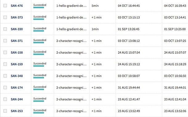
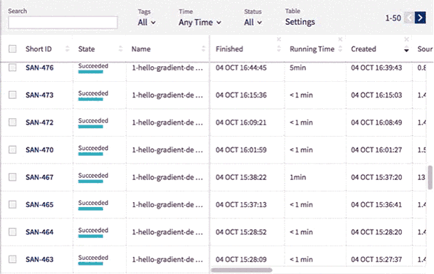
New Leaderboard
Use Neptune’s new leaderboard to organize data even more easily.
You can change the width of all columns and reorder them by simply drag and dropping their headings.
You can also edit the name, tags and notes directly in the table and display metadata including running time, worker type, environment, git hash, source code size and md5sum.
The experiments are now presented with their Short ID. This allows you to identify an experiment among those with identical names.
Sometimes you may want to see the same type of data throughout the entire project. You can now fix chosen columns on the left for quick reference as you scroll horizontally through the other sections of the table.
Parameters
Neptune comes with new, lightweight and yet more expressive parameters for experiments.
This means you no longer need to define parameters in configuration files. Instead, you just write them in the command line!
Let’s assume you have a script named main.py and you want to have 2 parameters: x=5 and y=foo . You need to pass them in the neptune send command:
neptune send -- '--x 5 --y foo'
Under the hood, Neptune will run python main.py –x 5 –y foo , so your parameters are placed in sys.argv . You can then parse these arguments using the library of your choice.
An example using argparse :
At deepsense.ai, we strive to make our mark on the cutting-edge research leading towards intelligent machines by providing practical machine learning tools and designs that make it much easier for scientists to track their experiments and verify novel ideas.
One particular step towards achieving this ideal was distributing a state-of-the-art Reinforcement Learning algorithm on a large CPU cluster, allowing super-fast training of agents that learned to master a wide range of Atari 2600 games. This post contains a brief description of our Distributed Deep Reinforcement Learning experiments. For a more in-depth look you can read our paper on the matter here.
Distributed reinforcement learning
Atari games are a widely accepted benchmark for deep reinforcement learning (RL). One common characteristic of these games is that they are very easy for humans to crack conceptually. Comparing the time it takes humans and computers to master these games can provide a clear indication of the capabilities of modern artificial intelligence. The first approaches to teach an agent to play Atari were developed by DeepMind and required around a week of training. The A3C algorithm developed later was able to achieve human performance in most games and did so with a similar amount of training time. But could computers ever learn faster than us?
Creating such a quick and bright Atari games learner would mean that computers outpaced us in understanding a game environment. The techniques that said agent would use to quickly develop a good grasp of the game could be studied to further develop our understanding of the cognitive features of a human brain. Moreover, faster training would give researchers considerably more flexibility in terms of experimenting and thus make verifying various RL approaches much quicker. Today, we present a Distributed Reinforcement Learning algorithm that efficiently trains on a large cluster of 64 12-core CPUs (768 cores in total). Our design enables agents to learn to play Atari games in as little as 20 minutes. We’re making our implementation available here.
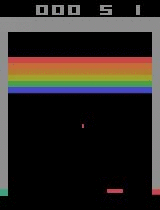
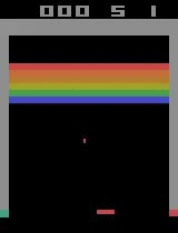
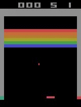
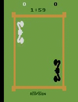
Breakout
Initial performance
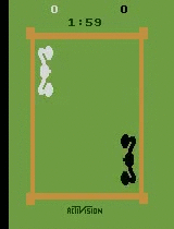
After 15 minutes of training
After 30 minutes of training
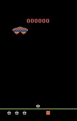
Assault
Initial performance
After 15 minutes of training
After 30 minutes of training
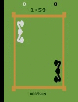
Boxing
Initial performance
After 15 minutes of training
After 30 minutes of training
Our achievement and results
By distributing the BA3C (details of single-machine implementation here) reinforcement learning algorithm, we were able to make an agent teach itself to play a wide range of Atari games rapidly, by just looking at a raw pixel output (game screen) from the game emulator. Our best experiments were distributed across 64 machines, each of which had 12 Intel CPU cores. In the game of Breakout, our agent achieves a superhuman score in just 20 minutes, which is a significant reduction of the single machine implementation learning time.
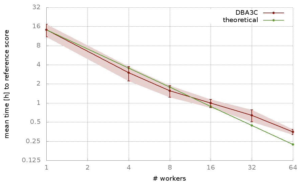
Training for Breakout on a single computer takes around 15 hours, bringing our implementation very close to the theoretical scaling (assuming computational power is maximized, using 64 times more CPUs should yield a 64-fold speed-up). The graph below shows the scaling of our implementation for different numbers of machines. Moreover, our algorithm exhibits robust results on many Atari environments, meaning that it is not only fast, but also adaptable to various learning tasks.
Graph showing the mean time of our algorithm (DBA3C) to achieve a score of 300 in the game of Breakout (average score of 300 needs to be obtained in 50 consecutive tries). The green line shows the theoretical scaling in reference to a single machine implementation.
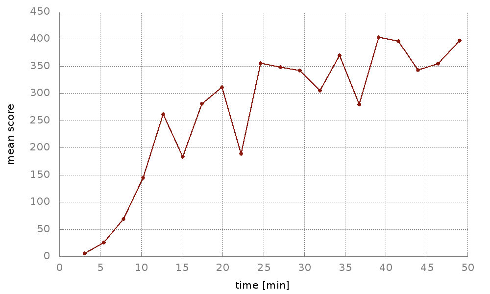
Using Neptune, a tool developed here at deepsense.ai, we were able to proactively track the performance of our agents. This enabled us to instantly verify if a certain feature of the algorithm works as expected. In Neptune, we could observe our agents’ real-time scores along with many other experiment-related metrics that we later used to optimize the algorithm. The graph below shows training curves from 10 different experiments on the Breakout game. Graphs were updated live in Neptune as the training went on.
A plot showing the live mean score obtained by the agent in 50 consecutive trials of Breakout
We managed to achieve very competitive training times. As we hope to inspire further research in the RL domain, we decided to open-source the implementation of our distributed reinforcement learning algorithm.
Details of the implementation
In the following section we describe the technicalities of our distributed set-up, aiming primarily to address a more advanced audience. To get the most out of our description, we recommend readers familiarize with this study done by the Google Brain team.
For parallelization we chose the synchronous paradigm. Synchronizing all our workers yielded much faster training times than the asynchronous set-up, where each node works for itself. Using a synchronous design prevented our model from using stale gradients in the updates, but at the same time introduced a problem known as slow stragglers. As suggested in the Google study linked above, deploying a few more backup workers can significantly reduce the impact of the slow stragglers, and doing just that has worked very well for us.
One of the biggest challenges that arises when dealing with largely distributed training is the cluster interconnect congestion on the parameter server nodes. Sending the gradients from multiple workers to a single parameter server bottlenecks the pipeline, effectively slowing down the training process.
To deal with that, we first reduced the model’s size. We noticed that a contraction of the neural network did not affect the accuracy of the algorithm, but did significantly increase the number of points processed per second, and hence also its speed.
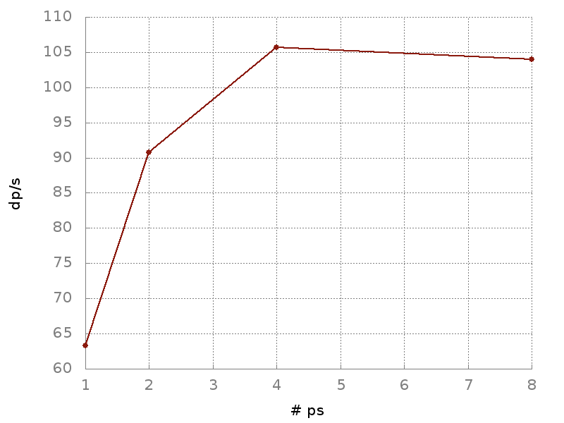
Since the communication overhead between the workers and parameter server was the biggest impeding factor to the speed of learning, we decided to balance the pressure on the pipeline by adding more parameter servers. This way, with the model weights distributed uniformly on multiple parameter servers, our training times began to pick up speed. The increase in processed data points per second for a different number of parameter servers can be seen below.
Graph showing the relation between the number of parameter servers and processed data-points per second – we can see that using more parameter servers significantly increases the dp/s
Related work
The distributed paradigm has been a topic of extensive research. Parallelization on 256 concurrent GPUs recently enabled a Facebook team to efficiently train the Resnet-51 model in one hour. Later developments from UC Berkeley reduced the time of training ImageNet to merely 24 minutes. The development of a distributed evolution strategy (ES) algorithm has led researchers from OpenAI to train agents to play Atari games in one hour by using 720 parallel CPUs. Since none of these designs have ever been applied to classical RL, the work done here can be considered pioneering in the field of distributed reinforcement learning.
Acknowledgements
The work on this distributed reinforcement learning design would not have been possible without the services of the PL-Grid supercomputing infrastructure, which provided us with all the computational power needed to conduct this research. We would like to thank Henryk Michalewski from the University of Warsaw for supervising the project and granting us access to the PL-Grid. We also used tensorpack, developed by Yuxin Wu, a very efficient open-source implementation of the A3C algorithm.
https://deepsense.ai/wp-content/uploads/2019/02/Solving-Atari-games-with-distributed-reinforcement-learning.jpg3371138Igor Adamskihttps://deepsense.ai/wp-content/uploads/2023/10/Logo_black_blue_CLEAN_rgb.pngIgor Adamski2017-10-04 10:00:002021-01-05 16:49:18Solving Atari games with distributed reinforcement learning