deepsense.ai
  • Careers
    • Job offers
    • Summer internship
  • Clients’ stories
  • Services
    • AI software
    • Team augmentation
    • AI discovery workshops
    • GPT and other LLMs fast track workshop
    • Generative AI
    • Train your team
  • Industries
    • Retail
    • Manufacturing
    • Financial & Insurance
    • IT operations
    • TMT & Other
    • Medical & Beauty
  • Knowledge base
    • deeptalks
    • Blog
    • R&D hub
  • About us
    • Our story
    • Management
    • Advisory board
    • Press center
  • Contact
  • Menu Menu
Playing Atari with deep reinforcement learning - deepsense.ai’s approach

Playing Atari on RAM with Deep Q-learning

September 27, 2016/in Data science, Deep learning, Machine learning /by Henryk Michalewski


In 2013 the Deepmind team invented an algorithm called deep Q-learning. It learns to play Atari 2600 games using only the input from the screen. Following a call by OpenAI, we adapted this method to deal with a situation where the playing agent is given not the screen, but rather the RAM state of the Atari machine. Our work was accepted to the Computer Games Workshop accompanying the IJCAI 2016 conference. This post describes the original DQN method and the changes we made to it. You can re-create our experiments using a publicly available code.

Atari games

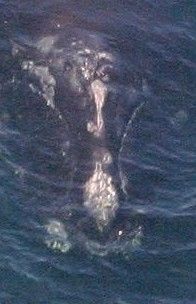
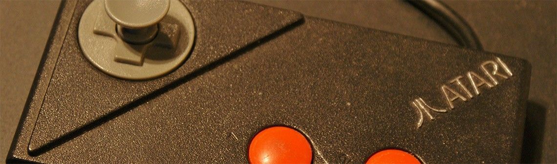
Atari 2600 is a game console released in the late 1970s. If you were a lucky teenager at that time, you would connect the console to the TV-set, insert a cartridge containing a ROM with a game and play using the joystick. Even though the graphics were not particularly magnificent, the Atari platform was popular and there are currently around \(400\) games available for it. This collection includes immortal hits such as Boxing, Breakout, Seaquest and Space Invaders.

Atari 2600 console

Atari 2600 console

Reinforcement Learning

We will approach the Atari games through a general framework called reinforcement learning. It differs from supervised learning (e.g. prediction what is represented in an image using Alexnet) and unsupervised learning (e.g. clustering, like in the nearest neighbours algorithm) because it utilizes two separate entities to drive the learning:

  1. agent (which sees states and rewards and decides on actions) and
  2. environment (which sees actions, changes states and gives rewards).
Richard S. Sutton and Andrew G. Barto: Reinforcement Learning: An Introduction

R. Sutton and A. Barto: Reinforcement Learning: An Introduction

In our case, the environment is the Atari machine, the agent is the player and the states are either the game screens or the machine’s RAM states. The agent’s goal is to maximize the discounted sum of rewards during the game. In our context, “discounted” means that rewards received earlier carry more weight: the first reward has a weight of \(1\), the second some \(gamma\) (close to \(1\)), the third \(gamma^2\) and so on.

Q-values

Q-value (also called action-value) measures how attractive a given action is in a given state. Let’s assume that the agent’s strategy (the choice of the action in a given state) is fixed. Then a Q-value of a state-action pair \((s, a)\) is the cumulative discounted reward the agent will get if it is in a state \(s\), executes the action \(a\) and follows his strategy from there on.
The Q-value function has an interesting property – if a strategy is optimal, the following holds:
$$
Q(s_t, a_t) = r_t + gamma max_a Q(s_{t+1}, a)
$$
One can mathematically prove that the reverse is also true. Namely, any strategy which satisfies the property for all state-action pairs is optimal. This fact is not restricted to deterministic strategies. For stochastic strategies, you have to add some expectation value signs and all the results still hold.

Q-learning

The above concept of Q-value leads to an algorithm learning a strategy in a game. Let’s slowly update the estimates of the state-action pairs to the ones that locally satisfy the property and change the strategy, so that in each state it will choose an action with the highest sum of expected reward (estimated as an average reward received in a given state after following given action) and biggest Q-value of the subsequent state.

for all (s,a):
    Q[s, a] = 0 #initialize q-values of all state-action pairs
for all s:
    P[s] = random_action() #initialize strategy
# assume we know expected rewards for state-action pairs R[s, a] and
# after making action a in state s the environment moves to the state next_state(s, a)
# alpha : the learning rate - determines how quickly the algorithm learns;
#                             low values mean more conservative learning behaviors,
#                             typically close to 0, in our experiments 0.0002
# gamma : the discount factor - determines how we value immediate reward;
#                               higher gamma means more attention given to far-away goals
#                               between 0 and 1, typically close to 1, in our experiments 0.95
repeat until convergence:
  1. for all s:
         P[s] = argmax_a (R[s, a] + gamma * max_b(Q[next_state(s, a), b]))
  2. for all (s, a):
         Q[s, a] = alpha*(R[s, a] + gamma * max_b Q[next_state(s, a), b]) + (1 - alpha)Q[s, a]

This algorithm is called Q-learning. It converges in the limit to an optimal strategy. For simple games like Tic-Tac-Toe, this algorithm, without any further modifications, solves them completely not only in theory but also in practice.

Deep Q-learning

Q-learning is a correct algorithm, but not an efficient one. The number of states which need to be visited multiple times to learn their action-values is too big. We need some form of generalization: when we learn about the value of one state-action pair, we can also improve our knowledge about other similar state-actions.
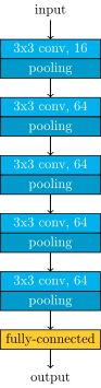
The deep Q-learning algorithm uses the convolutional neural network as a function approximating the Q-value function. It accepts the screen (after some transformations) as an input. The algorithm transforms the input with a couple of layers of nonlinear functions. Then it returns an up to \(18\) dimensional vector. Entries of the vector denote the approximated Q-values of the current state and each of the possible actions. The action to choose is the one with the highest Q-value.
Training consists of playing the episodes of the game, observing transitions from state to state (doing the currently best actions) and rewards. Having all this information, we can estimate the error, which is the square of the difference between the left- and right-hand side of the Q-learning property above:
$$
error = (Q(s_t, a_t) – (r_t + gamma max_a Q(s_{t+1}, a)))^2
$$
We can calculate the gradient of this error according to the network parameters and update them to decrease the error using one of the many gradient descent optimization algorithms (we used RMSProp).

DQN+RAM

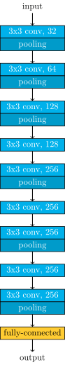
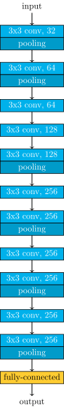
In our work, we adapted the deep Q-learning algorithm so that its input are not game screens, but the RAM states of the Atari machine. Atari 2600 has only \(128\) bytes of RAM. On one hand, this makes our task easier, as our input is much smaller than the full screen of the console. On the other hand, the information about the game may be hard to retrieve. We tried two network architectures. One with \(2\) hidden ReLU layers, \(128\) nodes each, and the other with \(4\) such layers. We obtained results comparable (in two games higher, in one lower) to those achieved with the screen input in the original DQN paper. Admittedly, higher scores can be achieved using more computational resources and some additional tricks.

Tricks

The method of learning Atari games, as presented above and even with neural networks employed to approximate the Q-values, would not yield good results. To make it work, the original DQN paper’s authors and we in our experiments, employed a few improvements to the basic algorithm. In this section, we discuss some of them.

Epsilon-greedy strategy

When we begin our agent’s training, it has little information about the value of particular game states. If we were to completely follow the learned strategy at the start of the training we’d be nearly randomly choosing some actions to follow in the first game states. As the training continues, we’d stick to these actions for the first states, as their value estimation would be positive (and for the other actions would be nearly zero). The value of the first-chosen action would improve and we’d only pick these, without even testing the other possibilities. The first decisions, made with little information, would be reinforced and followed in the future.
We say that such a policy doesn’t have a good exploration-exploitation tradeoff. On one hand, we’d like to focus on the actions that led to reasonable results in the past, but on the other ahnd, we prefer our policies to extensively explore the state-action space.
The solution to this problem used in DQN is using an epsilon-greedy strategy during training. This means that at any time with some small probability \(varepsilon\) the agent chooses a random action, instead of always choosing the action with the best Q-value in the given state. Then, every action will get some attention and its state-action value estimation will be based on some (possibly limited) experience and not the initialization values.
We join this method with epsilon decay — at the beginning of training we set \(varepsilon\) to a high value (\(1.0\)), meaning that we prefer to explore the various actions and gradually decrease \(varepsilon\) to a small value, that indicate the preference to exploit the well-learned action-values.

Experience replay

Another trick used in DQN is called experience replay. The process of training a neural network consist of training epochs; in each epoch we pass all the training data, in batches, as the network input and update the parameters based on the calculated gradients.
When training reinforcement learning models, we don’t have an explicit dataset. Instead, we experience some states, actions, and rewards. We pass them to the network, so that our statistical model can learn what to do in similar game states. As we want to pass a particular state/action/reward tuple multiple times to the network, we save them in memory when they are seen. To fit this data to the RAM of our GPU, we store at most \(100 000\) recently observed state/action/reward/next state tuples.
When the dataset is queried for a batch of training data, we don’t return consecutive states, but a set of random tuples. This reduces correlation between states processed in a given step of learning. As a result, this improves the statistical properties of the learning process.
For more details about experience replay you can see Section 3.5 of Lin’s thesis. As quite a few other tricks in reinforcement learning, this method was invented back in 1993 – significantly before the current deep learning boom.

Frameskip

Atari 2600 was designed to use an analog TV as the output device. The console generated \(60\) new frames appearing on the screen every second. To simplify the search space we imposed a rule that one action is repeated over a fixed number of frames. This fixed number is called the frame skip. The standard frame skip used in the original work on DQN is \(4\). For this frame skip the agent makes a decision about the next move every \( 4cdot frac{1}{60} = frac{1}{15}\) of a second. Once a decision is made, it remains unchanged during the next \(4\) frames. A low frame skip allows the network to learn strategies based on a super-human reflex. A high frame skip will limit the complexity of a strategy. Hence learning may be faster and more successful whenever strategy matters over tactic. In our work , we tested frame skips equal to \(4,8\) and \(30\).

Further research

We are currently testing other strategy-learning algorithms on a Xeon Phi architecture.

https://deepsense.ai/wp-content/uploads/2019/02/Playing-Atari-games-using-RAM-state.jpg 337 1140 Henryk Michalewski https://deepsense.ai/wp-content/uploads/2019/04/DS_logo_color.svg Henryk Michalewski2016-09-27 12:00:342023-02-28 21:57:21Playing Atari on RAM with Deep Q-learning
Neptune - Machine Learning Platform

Neptune – Machine Learning Platform

September 26, 2016/in Data science, Deep learning, Machine learning, Neptune /by Rafał Hryciuk

In January 2016, deepsense.ai won the Right Whale Recognition contest on Kaggle. The competition’s goal was to automate the right whale recognition process using a dataset of aerial photographs of individual whales. The terms and conditions for the competition stated that to collect the prize, the winning team had to provide source code and a description of how to recreate the winning solution. A fair request, but as it turned out, the winning solution’s authors spent about three weeks recreating all of the steps that led them to the winning machine learning model.

When data scientists work on a problem, they need to test many different approaches – various algorithms, neural network structures, numerous hyperparameter values that can be optimized etc. The process of validating one approach can be called an experiment. The inputs for every experiment include: source code, data sets, hyperparameter values and configuration files. The outputs of every experiment are: output model weights (definition of the model), metric values (used for comparing different experiments), generated data and execution logs. As we can see, that’s a lot of different artifacts for each experiment. It is crucial to save all of these artifacts to keep track of the project – comparing different models, determining which approaches were already tested, expanding research from some experiment from the past etc. Managing the process of experiment executions is a very hard task and it is easy to make a mistake and lose an important artifact.
To make the situation even more complicated, experiments can depend on each other. For example, we can have two different experiments training two different models and a third experiment that takes these two models and creates a hybrid to generate predictions. Recreating the best solution means finding the path from the original data set to the model that gives the best results.

Recreating the path that led to the best model

The deepsense.ai research team performed around 1000 experiments to find the competition-winning solution. Knowing all that, it becomes clear why recreating the solution was such a difficult and time consuming task.
The problem of recreating a machine learning solution is present not only in an academic environment. Businesses struggle with the same problem. The common scenario is that the research team works to find the best machine learning model to solve a business problem, but then the software engineering team has to put the model into a production environment. The software engineering team needs a detailed description of how to recreate the model.
Our research team needed a platform that would help them with these common problems. They defined the properties of such a platform as:

  • Every experiment and the related artifacts are registered in the system and accessible for browsing and comparing;
  • Experiment execution can be monitored via real-time metrics;
  • Experiment execution can be aborted at any time;
  • Data scientists should not be concerned with the infrastructure for the experiment execution.

deepsense.ai decided to build Neptune – a brand new machine learning platform that organizes data science processes. This platform relieves data scientists of the manual tasks related to managing their experiments. It helps with monitoring long-running experiments and supports team collaboration. All these features are accessible through the powerful Neptune Web UI and useful for scripting CLI.
Neptune - Machine Learning Platform Logo
Neptune is already used in all machine learning projects at deepsense.ai. Every week, our data scientists execute around 1000 experiments using this machine learning platform. Thanks to that, the machine learning team can focus on data science and stop worrying about process management.

Experiment Execution in Neptune

Main Concepts of the Machine Learning Platform

Job

A job is an experiment registered in Neptune. It can be registered for immediate execution or added to a queue. The job is the main concept in Neptune and contains a complete set of artifacts related with the experiment:

  • source code snapshot: Neptune creates a snapshot of the source code for every job. This allows a user to revert to any job from the past and get the exact version of the code that was executed;
  • metadata: name, description, project, owner, tags;
  • parameters: customly defined by a user. Neptune supports boolean, numeric and string types of parameters;
  • data and logs generated by the job;
  • metric values represented as channels.

Neptune is library and framework agnostic. Users can leverage their favorite libraries and frameworks with Neptune. At deepsense.ai we currently execute Neptune jobs that use: TensorFlow, Theano, Caffe, Keras, Lasagne or scikit-learn.

Channel

A channel is a mechanism for real-time job monitoring. In the source code, a user can create channels, send values through them and then monitor these values live using the Neptune Web UI. During job execution, a user can see how his or her experiment is performing. The Neptune machine learning platform supports three types of channels:

  • Numeric: used for monitoring any custom-defined metric. Numeric channels can be displayed as charts. Neptune supports dynamic chart creation from the Neptune Web UI with multiple channels displayed in one chart. This is particularly useful for comparing various metrics;
  • Text: used for logs;
  • Image: used for sending images. A common use case for this type of channel is checking the behavior of an applied augmentation when working with images.
Neptune - Machine Learning Platform, Comparing two Neptune image channels
Comparing two Neptune image channels

Queue

A queue is a very simple mechanism that allows a user to execute his or her job on remote infrastructure. A common setup for many research teams is that data scientists develop their code on local machines (laptops), but due to hardware requirements (powerful GPU, large amount of RAM, etc) code has to be executed on a remote server or in a cloud. For every experiment, data scientists have to move source code between the two machines and then log into the remote server to execute the code and monitor logs. Thanks to our machine learning platform, a user can enqueue a job from a local machine (the job is created in Neptune, all metadata and parameters are saved, source code copied to users’ shared storage). Then, on a remote host that meets the job requirements the user can execute the job with a single command. Neptune takes care of copying the source code, setting parameters etc.
The queue mechanism can be used to write a simple script that queries Neptune for enqueued jobs and execute the first job from the queue. If we run this script on a remote server in an infinite loop, we don’t have to log to the server ever again because the script executes all the jobs from the queue and reports the results to the machine learning platform.

Creating a Job

Neptune is language and framework agnostic. A user can communicate with Neptune using REST API and Web Sockets from his or her source code written in any language. To make the communication easier, we provide a high-level client library for Python (other languages are going to be supported soon).
Let’s examine a simple job that provided with amplitude and sampling_rate generates sine and cosine as functions of time (in seconds).

import math
import time
from deepsense import neptune
ctx = neptune.Context()
amplitude = ctx.params.amplitude
sampling_rate = ctx.params.sampling_rate
sin_channel = ctx.job.create_channel(name='sin', channel_type=neptune.ChannelType.NUMERIC)
cos_channel = ctx.job.create_channel(name='cos', channel_type=neptune.ChannelType.NUMERIC)
logging_channel = ctx.job.create_channel(name='logging', channel_type=neptune.ChannelType.TEXT)
ctx.job.create_chart(name='sin & cos chart', series={'sin': sin_channel, 'cos': cos_channel})
ctx.job.finalize_preparation()
# The time interval between samples.
period = 1.0 / sampling_rate
# The initial timestamp, corresponding to x = 0 in the coordinate axis.
zero_x = time.time()
iteration = 0
while True:
    iteration += 1
    # Computes the values of sine and cosine.
    now = time.time()
    x = now - zero_x
    sin_y = amplitude * math.sin(x)
    cos_y = amplitude * math.cos(x)
    # Sends the computed values to the defined numeric channels.
    sin_channel.send(x=x, y=sin_y)
    cos_channel.send(x=x, y=cos_y)
    # Formats a logging entry.
    logging_entry = "sin({x})={sin_y}; cos({x})={cos_y}".format(x=x, sin_y=sin_y, cos_y=cos_y)
    # Sends a logging entry.
    logging_channel.send(x=iteration, y=logging_entry)
    time.sleep(period)

The first thing that we can see is that we need to import Neptune library and create a neptune.Context object. The Context object is an entrypoint for Neptune integration. Afterwards, using the context we obtain values for job parameters: amplitude and sampling_rate.
Then, using neptune.Context.job we create numeric channels for sending sine and cosine values and a text channel for sending logs. We want to display sin_channel and cos_channel on a chart, so we use neptune.Context.job.create_chart to define a chart with two series named sin and cos. After that, we need to tell Neptune that the preparation phase is over and we are starting the proper computation. That is what: ctx.job.finalize_preparation() does.
In an infinite loop we calculate sine and cosine functions values and send these values to Neptune using the channel.send method. We also create a human-readable log and send it through logging_channel.
To run main.py as a Neptune job we need to create a configurtion file – a descriptor file with basic metadata for the job.

name: Sine-Cosine Generator
project: Trigonometry
owner: Your Name
parameters:
  - name: amplitude
    type: double
    default: 1.0
    required: false
  - name: sampling_rate
    type: double
    default: 2
    required: false

config.yaml contains basic information about the job: name, project, owner and parameter definitions. For our simple Sine-Cosine Generator we need two parameters of double type: amplitude and sampling_rate (we already saw in the main.py how to obtain parameter values in the code).
To run the job we need to use the Neptune CLI command:
neptune run main.py –config config.yaml –dump-dir-url my_dump_dir — –amplitude 5 –sampling_rate 2.5
For neptune run we specify: the script that we want to execute, the configuration for the job and a path to a directory where snapshot of the code will be copied to. We also pass values of the custom-defined parameters.

Job Monitoring

Every job executed in the machine learning platform can be monitored in the Neptune Web UI. A user can see all useful information related to the job:

  • metadata (name, description, project, owner);
  • job status (queued, running, failed, aborted, succeeded);
  • location of the job source code snapshot;
  • location of the job execution logs;
  • parameter schema and values.
Neptune – Machine Learning Platform, Parameters for Sine-Cosine Generator
Parameters for Sine-Cosine Generator

A data scientist can monitor custom metrics sent to Neptune through the channel mechanism. Values of the incoming channels are displayed in the Neptune Web UI in real time. If the metrics are not satisfactory, the user can decide to abort the job. Aborting the job can also be done from the Neptune Web UI.

Neptune – Machine Learning Platform, Channels for Sine-Cosine Generator
Channels for Sine-Cosine Generator
Neptune – Machine Learning Platform, Comparing values of multiple metrics using Neptune channels
Comparing values of multiple metrics using Neptune channels

Numeric channels can be displayed graphically as charts. A chart representation is very useful to compare various metrics and to track changes of metrics during job execution.

Neptune – Machine Learning Platform, Chart for Sine-Cosine Generator
Chart for Sine-Cosine Generator
Neptune – Machine Learning Platform, Charts displaying custom metrics
Charts displaying custom metrics

For every job a user can define a set of tags. Tags are useful for marking significant differences between jobs and milestones in the project (i.e if we are doing a MINST project, we can start our research by running the job with a well known and publicly available algorithm and tag it ‘benchmark’).

Comparing Results and Collaboration

Every job executed in the Neptune machine learning platform is registered and available for browsing. Neptune’s main screen shows a list of all executed jobs. User can filter jobs using job metadata, execution time and tags.

Neptune – Machine Learning Platform, Neptune jobs list
Neptune jobs list

A user can select custom-defined metrics to show as columns on the list. The job list can be sorted using values from every column. That way, a user can select which metric he or she wants to use for comparison, sort all jobs using this metric and then find the job with the best score.
Thanks to a complete history of job executions, data scientists can compare their jobs with jobs executed by their teammates. They can compare results, metrics values, charts and even get access to the snapshot of code of a job they’re interested in.
Thanks to Neptune, the machine learning team at deepsense.ai was able to:

  • get rid off spreadsheets for keeping history of executed experiments and their metrics values;
  • eliminate sharing source code across the team as an email attachment or other innovative tricks;
  • limit communication required to keep track of project progress and achieved milestones;
  • unify visualisation for metrics and generated data.

Join the Early Adopters Program

Apply for our Early Adopters Program and get early access to Neptune – Machine Learning Platform.
Benefits of joining the program include:

  • You will be one of the first to get full access to this innovative product designed especially for data scientists for FREE;
  • You will have direct impact on future product features;
  • You will get support from our team of engineers;
  • You can share your ideas with our experts and the community of the world’s leading data scientists.
https://deepsense.ai/wp-content/uploads/2019/02/neptune-machine-learning-platform.jpg 217 750 Rafał Hryciuk https://deepsense.ai/wp-content/uploads/2019/04/DS_logo_color.svg Rafał Hryciuk2016-09-26 11:48:132021-01-05 16:50:56Neptune – Machine Learning Platform
Which whale is it, anyway? Face recognition for right whales using deep learning

Which whale is it, anyway? Face recognition for right whales using deep learning

January 16, 2016/in Data science, Deep learning, Machine learning /by Robert Bogucki

noaa_fisheries_smallRight Whale Recognition was a computer vision competition organized by the NOAA Fisheries on the Kaggle.com data science platform. Our machine learning team at deepsense.ai has finished 1st! In this post we describe our solution.

The challenge

The goal of the competition was to recognize individual right whales in photographs taken during aerial surveys. When visualizing the scenario, do not forget that these giants grow up to more than 18 metres, and weigh up to 91 tons. There were 447 different right whales in the data set (and this is likely the overall number of living specimens). Even though that number is (terrifyingly) small for a species, uniquely identifying a whale poses a significant challenge for a person. Automating at least some parts of the process would be immensely beneficial to right whales’ chances of survival.

“Recognizing a whale in real-time would also give researchers on the water access to potentially life-saving historical health and entanglement records as they struggle to free a whale that has been accidentally caught up in fishing gear,”

— excerpt from competition’s description page.

The photographs had been taken at different times of day, and with various equipment. They ranged from very clear and centered on the animal to taken from afar and badly focused.

w_4615 w_4661 w_10578 w_10579 w_81 w_4771
A non-random sample from the dataset

The teams were expected to build a model that recognizes which one of the 447 whales is captured in the photograph. More technically, for each photo, we were asked to provide a probability distribution over all 447 whales. The solutions were judged by multiclass log loss, also known as cross-entropy loss.
It is worth noting that the dataset was not balanced. The number of pictures per whale varied a lot: there were some “celebrities” having around forty, a great deal with over a dozen, and around twenty with just a single photo! Another challenge, is that images representing different classes (i.e. different whales) were very similar to each other. This is somewhat different than the situation where we try to discriminate between, say, dogs, cats, wombats and planes. This posed some difficulties for the neural networks that we had been training – the unique characteristics that make up an individual whale, or that set this particular whale apart from others, occupy only a small portion of an image and are not very apparent. Helping out our classifiers to focus on the correct features, i.e. the whale’s heads and their callosity patterns, turned out to be crucial.

Related:  Playing Atari with deep reinforcement learning - deepsense.ai’s approach

The backbone of our solution

Convolutional neural networks (CNNs) have proven to do extraordinarily well in image recognition tasks, so it was natural for us to base our solution on them. In fact, to our knowledge, all top contestants have used them almost at every step. Even though some say that those techniques require huge amounts of data (and we only had 4,544 training images available with some of the whales appearing only once in the whole training set), we were still able to produce a well-performing model, proving that CNNs are a powerful tool even on limited data.
In fact our solution consisted of multiple steps:
– head localizer (using CNNs),
– head aligner (using CNN),
– training several CNNs on passport-like photos of whales (obtained from previous steps),
– averaging and tuning the predictions (not using CNNs).
One additional trick that has served us well is providing the networks with some additional targets, even though those additional targets were not necessarily used afterwards or required in any way. If the additional targets depend on the part of image that is of particular interest for us (i.e. head and callosity pattern in this case), this trick should force the network to focus on this area. Also, the networks have more stimuli to learn on, and thus have to develop more robust features (sensible for more than one task) which should limit overfitting.

Software and hardware

We used Python, NumPy and Theano to implement our solution. To create manual annotations (and do not lose sanity during these long moments of questionable joy) we employed Sloth (a universal labeling tool), as well as an ad-hoc Julia script.
To train our models we used two types of Nvidia GPUs: Tesla K80 and GRID K520.

Domain knowledge

Even though it seems significantly harder for humans to identify whales than other people, neural networks do not suffer from such problem for obvious reasons. Even then, a bit of Wikipedia research on right whales reveals that “the most distinguishing feature of a right whale is the rough patches of skin on its head which appear white due to parasitism by whale lice.” Turns out that it not only distinguishes them from other species of whales, but also serves as an excellent way to differentiate between specimens. Our solution uses this fact to great lengths. Besides this somewhat trivial hint (provided by the organizers) about what to look at, we (sadly) posses no domain knowledge about right whales.

Preparing for the take-off

Before going further into the details, a disclaimer is needed. During a competition, one is (or should be) more tempted to test new approaches, than to fine tune and clean up existing ones. Hence, soon after an idea had proved to work well enough, we usually settled on it and left it “as is”. As a side-effect, we expect that some parts of the solution may possess unnecessary artifacts or complexity that could (and ought to) be eliminated. Nevertheless, we have not done so during the competition, and decided not to do so here either.
One does not need to see many images from the dataset in order to realize that whales do not pose very well (or at least were reluctant to do so in this particular case).

w_12w_7
Not very cooperative whales

Therefore, before training final classifiers we spent some time (and energy) to account for this fact. The general idea of this approach can be thought of as obtaining a passport photo from a random picture where the subject is in some arbitrary position. This boiled down to training a head localizer and a head aligner. The first one takes a photo and produces a bounding box around the head, still the head may be arbitrarily rotated and not necessarily in the middle of the photo. The second one takes a photo of the head and aligns and rescales it, so that the blowhead and bonnet-tip are always in the same place, and the distance between them is constant. Both of these steps were done by training a neural network on manual annotations for the training data.

w_0_indygo2
Bonnet-tip (red) and blowhead (blue)

Localizing the whale

This was the first step in order to achieve good quality, passport-like photos. In order to obtain the training data, we have manually annotated all the whales in the training data with bounding boxes around their heads (a special thanks goes to our HR department for helping out!).

w_0_bboxBounding box produced by the head localizer

These annotations amounted to providing four numbers for each image in the training set: coordinates of the bottom-left and the top-right points of the rectangle. We then proceeded to train a CNN which takes an original image (resized to 256×256) and outputs the two coordinates of the bounding box. Although this is clearly a regression task, instead of using L2 loss, we had more success with quantizing the output into bins and using Softmax together with cross-entropy loss. We have also tried several different approaches, including training a CNN to discriminate between head photos and non-head photos or even some unsupervised approaches. Nevertheless, their results were inferior.
In addition, the head localizing network also had to predict the coordinates of the blowhead and bonnet-tip (in the same, quantized manner), however it was less successful in this task, so we ignored this output.
We trained 5 different networks, all of them had almost the same architecture.

gscp_smallerHead localizer’s architecture

Where they differed is the number of buckets used to quantize the coordinates. We have tried 20, 40, 60, 128, and also another (a little bit smaller) network using 20 buckets.
Before feeding the image into the network, we had used the following data augmentation (after resizing it to 256×256):
– rotation: up to 10° (note that if you allow bigger angles, it won’t be enough to simply rotate the points – you’ll have to implement some logic to recalculate the bounding box – we were too lazy to do this),
– rescaling: random ratio between 1/1.2 and 1.2,
– colour perturbation (as in Krizhevsky et al. 2012), with scale 0.01.
Although we have not used test-time augmentation here, we combined the outputs from all the 5 networks. Each time a crop was passed to the next step (head alignment), a random one from all 5 variants was chosen. As can be seen above, the crops provided by these networks were quite satisfactory. To be honest – we did not really “physically” crop the images (i.e. produce a bunch of smaller images). What we’ve done instead, and what turned out to be really handy, is producing a json file with the coordinates of bounding boxes. This may seem trivial, but doing so encouraged and allowed us to easily experiment with them.

Related:  Logo detection and brand visibility analytics - example

”Passport photos” of whales

The final step of this “make the classifier’s life easier” pipeline was to align the photos so that they all conform to the same standards. The idea was to train a CNN that estimates the coordinates of blowhead and bonnet-tip. Having them, one can easily come up with a transformation that maps the original image into one where these two points are always in the same position. Thanks to the annotations made by Anil Thomas, we had the coordinates for the training set. So, once again we proceeded to train CNN to predict quantized coordinates. Although we do not claim that it was impossible to pinpoint these points using the whole image (i.e. avoid the previous step), we now face a possibly easier task – we know the approximate location of the head.
In addition, the network had some additional tasks to solve! First of all it needed to predict which whale is on the image (i.e. solve the original task). Moreover, it needed to tell whether the callosity pattern on the whale’s head is continuous or not (training on manual annotations once again, although there was much less work this time since looking at 2-3 images per whale was enough).

w_8734_non_continuous
w_1000_continuous

Broken (left) and continuous (right) callosity patterns

We used the following architecture.

new_gscHead aligner’s architecture

As an input to head aligner we took the crops from the head localizer. This time we dared to use a more bold augmentation:
– translation: random up to 4 pixels,
– rotation: up to 360°,
– rescaling: random ratio between 1.0 and 1.5,
– random flip,
– colour perturbation with scale 0.01.
Also, we used test-time augmentation – the results were averaged over 5 random augmentations (not much, but still!). This network achieved surprisingly good results. To be more (or less) accurate – during manual inspection, the blowhead and bonnet-tip positions were predicted almost perfectly for almost all images. Besides, as a by-product (or was it the other way?), we started to see some promising results for the original task of identifying the whales. The (quite pessimistic) validation loss was around 2.2.

Putting everything together

When chaining multiple machine learning algorithms in the pipeline, some caution is needed. If we train a head localizer and head aligner on the training data and use them to produce “passport photos” for both the training and testing set, we may end up with photos that vastly differ in quality (and possibly some other properties). This can turn out to be a serious difficulty when training a classifier on top of these crops – if at test time it faces inputs that don’t bear any similarity to those it was accustomed to, it does not perform.
Although we were aware of this fact, when inspecting the crops we discovered that the quality did not differ much between training and testing data. Moreover, we’ve seen a huge improvement in the log loss. Following the mindset of “more ideas, less dwelling”, we decided to settle on this impure approach and press on.

img_1_w_8604_class_idx_349 img_2_w_1354_class_idx_322 img_1_w_7356_class_idx_67 img_1_w_3178_class_idx_332 img_1_w_929_class_idx_51 img_1_w_427_class_idx_372

“Passport photos” of whales

Final classifier

Network architecture

Almost all of our models worked on 256×256 images and shared the same architecture. All convolutional layers had 3×3 filters and did not change the size of the image, all pooling layers were 3×3 with 2 stride (they halved the size). In addition all convolutional layers were followed by batch normalization and ReLU nonlinearity.

new_gsc3Main net’s architecture

In the final blend, we have also used a few networks with an analogous architecture, but working on 512×512 images, and one network with a “double” version of this architecture (with an independent copy of the stacked convolutional layers, merged just before the fully-connected layer).
Once again, we’ve violated the networks’ comfort zone by adding an additional target – determining the continuity of the callosity pattern (same as in the head aligner case). We’ve also tried adding more targets coming from other manual annotations, one such target was “how much was the face symmetric”. Unfortunately, it did not improve the results any further.

Data augmentation

At this point data augmentation is a little bit trickier than usual. The reason behind this, is that you have to balance between enriching the dataset enough, and not ruining the alignment and normalization obtained from the previous step. We ended up using quite mild augmentation. Although the exact parameters were not constant among all models, the most common were:
– translation: random up to 4 pixels,
– rotation: up to 8°,
– rescaling: random ratio between 1.0 and 1.3,
– random flip,
– colour perturbation with scale 0.01.
We also used test-time augmentation, and averaged over 20+ random augmentations.

Initialization

We used a very simple initialization rule, a zero-centred normal distribution with std 0.01 for convolutional layers and std 0.001 for fully connected layers. This has worked well enough.

Regularization

For all models, we have used only L2 regularization. However, separate hyperparameters were used for convolutional and fully connected layers. For convolutional layers, we used a smaller regularization, around 0.0005, while for fully connected ones we preferred higher values, usually around 0.01 – 0.05.
One should also recall that we were adding supplementary targets to the networks. This imposes additional constraints on weights, enforces more focus on the head of the whale (instead of, say, some random patterns on the water), i.e. it works against overfitting.

Training

We trained almost all of our models with stochastic gradient descent (SGD) combined with 0.9 momentum. Usually we settled after around 500-1000 epochs (the exact moment didn’t really matter much, because the lack of overfitting). During the training process we used quite slow exponential decay on the learning rate (0.9955) and also manually adjusted the learning rate from time to time. After a rough kick – increasing the learning rate (yet still leaving the decay) the network’s error (on both: training and validation) went up a lot. Yet it tended to settle on a lower error after a few epochs to get back on a good track. Our best model also uses another idea – it was first trained with Nesterov momentum for over a hundred epochs, and then we switched to using Adam (adaptive moment estimation). We couldn’t achieve similar loss when using Adam all the way from the start. The initial learning rate may not have mattered much, but we used values around 0.0005.

Validation

We used a random 10% of the training data for validation. Thanks to our favourite seed 7300, we kept it the same for all models. Although, we were aware that this method caused some whales to be absent in the training set, it has worked good enough. The validation loss was quite pessimistic, and correlated well with the leaderboard.
Giving up 10% of a relatively small dataset is not something one would decide to do without any hesitation. Therefore, after we had decided that a model is good enough to use it, we proceeded to reuse the validation set for training (it was straightforward because we didn’t have any problems with overfitting). This was done either by a time-consuming process of rerunning everything from scratch on the whole training set (rarely), or (more often) adding the validation set to the training one and running 50-100 additional epochs. This was also meant to curate the issue of single-photo-whales appearing only in our validation set.

Combining the predictions

We have ended up with a number of models scoring in a range of 0.97 to 1.3 according to our validation (actual test scores were actually better). Thanks to keeping a consistent validation set we were able to test some blending techniques as well as basic transformations. We have concluded that using more complex ensembling methods would not be plausible due to the fact that our validation set did not include all the distinct whales, and was, in fact, quite small. Having no time left for some fancy cross-validation like ensembling, we settled on something ad-hoc and simple.
Even though simple weighted average of the predictions did not provide a better score than the best model alone (unless we increased the best model’s weight significantly), it performed better when combined with a simple transformation of raising the predictions to a moderate power (in the final solution we used 1.45). This translated into roughly ~0.1 improvement in the log loss. We have not scrutinized this enough, yet one may hypothesize that this trick worked because our fully connected layers were strongly regularized, and were reluctant to produce more extreme probabilities.
We also used some “safety” transformations, namely increasing all the predictions by a certain epsilon as well as slightly skewing them to the whale distribution found in the training set. They had not impacted our score much.

Loading images

At the latest, and middle stages of our solution the images we loaded from the disk were original ones. They are quite big. To efficiently use the gpu we had to load them in parallel. We thought the main cost was loading the images from the disk. It turned out not to be true. Conversely, it was decoding JPEG file to a numpy array. We did a quick and dirty benchmark, with 111 random original images from the dataset, 85Mb total. Reading them, when they are not cached in RAM takes ~420 ms. Whereas reading, and decoding to numpy arrays takes ~10 seconds. That’s a huge difference. The possible solutions to mitigate this, might be using other image formats, that offer better encoding speeds (at the cost of image sizes), decoding at GPU, etc.

What might have made it tick

Although, it’s hard to pinpoint a single trick or technique that overshadows everything else (and to do so, one needs a more careful analysis), we have hypothesized about the key tricks.

Producing good quality crops with well aligned heads

We have achieved this by doing this in two stages, and the results were vastly superior than what we observed with just a single stage.

Manual labour and providing the networks with additional targets

This was based on adding additional annotations to the original images. It required manual inspection of thousands of whales images, but we ended up using them in all stages (head localizing, head aligning, and classification).

Kicking the learning rate

Although it might have been the combination of a little bit careless initialization, poor learning rate decay schedule, and not fancy enough SGD, it turned out, that kicking (increasing) the learning rate did a great job.

Screenshot from 2016-01-15 15:33:58Loss functions after kicking the learning rate


Calibrating the probabilities

Almost all our models, and blends of models benefitted from raising the predictions to a moderate power in the range [1.1 – 1.6]. This trick, discovered at the end of the competition, improved the score by ~0.1.

Reusing the validation set

Merging validation and training sets and running for additional 50-100 epochs gave us steady improvements on the score.

Related:  Region of interest pooling explained

Conclusion

Overall, this was an amazing problem to tackle and an amazing competition to take part in. We have learned a lot during the process, and are actually quite amazed with the super-powers of deep learning!
A special thanks to Christin Khan and NOAA for presenting the data science community with this exceptional challenge. We hope that this will inspire others. Of course, all this would be much harder without Kaggle.com, which does a great job with their platform. We would also like to thank Nvidia for giving us access to Nvidia K80 GPUs – they’ve done a great job.

Robert Bogucki
Marek Cygan
Maciej Klimek
Jan Kanty Milczek
Marcin Mucha

https://deepsense.ai/wp-content/uploads/2016/01/deep-learning-right-whale-recognition-kaggle.jpg 337 1140 Robert Bogucki https://deepsense.ai/wp-content/uploads/2019/04/DS_logo_color.svg Robert Bogucki2016-01-16 16:16:562021-01-05 16:51:52Which whale is it, anyway? Face recognition for right whales using deep learning
Diagnosing diabetic retinopathy with deep learning

Diagnosing diabetic retinopathy with deep learning

September 3, 2015/in Data science, Deep learning, Machine learning /by Robert Bogucki

What is the difference between these two images?


The one on the left has no signs of diabetic retinopathy, while the other one has severe signs of it.

If you are not a trained clinician, the chances are, you will find it quite hard to correctly identify the signs of this disease. So, how well can a computer program do it?
In July, we took part in a Kaggle competition, where the goal was to classify the severity of diabetic retinopathy in the supplied images of retinas.
As we’ve learned from the organizers, this is a very important task. Diabetic retinopathy is the leading cause of blindness in the working-age population of the developed world. It is estimated to affect over 93 million people.
The contest started in February, and over 650 teams took part in it, fighting for the prize pool of $100,000.
The contestants were given over 35,000 images of retinas, each having a severity rating. There were 5 severity classes, and the distribution of classes was fairly imbalanced. Most of the images showed no signs of the disease. Only a few percent had the two most severe ratings.
The metric with which the predictions were rated was a quadratic weighted kappa, which we will describe later.
The contest lasted till the end of July. Our team scored 0.82854 in the private standing, which gave us 6th place. Not too bad, given our quite late entry.
You can see our progress on this plot:
xxx
Also, you can read more about the competition here.

Solution overview

What should be no surprise in an image recognition task, most of the top contestants used deep convolutional neural networks (CNNs), and so did we.
Our solution consisted of multiple steps:

  • image preprocessing
  • training multiple deep CNNs
  • eye blending
  • kappa score optimization

We briefly describe each of these steps below. Throughout the contest we used multiple methods for image preprocessing and trained many nets with different architectures. When ensembled together, the gain over the best preprocessing method and the best network architecture was little. We therefore limited ourselves to describing the single best model. If you are not familiar with convolutional networks, check out this great introduction by Andrej Karpathy: http://cs231n.github.io/convolutional-networks/.

Preprocessing

The input images, as provided by the organizers, were produced by very different equipment, had different sizes and very different colour spectrum. Most of them were also way too large to perform any non-trivial model fitting on them. A minimum preprocessing to make network training possible is to standardize the dimensions, but ideally one would want to normalize all other characteristics as well. Initially, we used the following simple preprocessing steps:

  • Crop the image to the rectangular bounding box containing all pixels above a certain threshold
  • Scale it to 256×256 while maintaining the aspect ratio and padding with black background (the raw images have black background as well, more or less)
  • For each RGB component separately, remap the colour intensities so that the CDF (cumulative distribution function) looks as close to linear as possible (this is called “histogram normalization”)

All these steps can be achieved in a single call of ImageMagick’s command line tool. In time, we realized that some of the input images contain regions of rather intensive noise. When using the simple bounding-box cropping described above, this leads to very bad quality crops, i.e. the actual eye occupying an arbitrary and rather small part of the image.
noise
You can see gray noise at the top of the image. Using state of the art edge detectors, e.g. Canny, did not help much. Eventually, we developed a dedicated cropping procedure. This procedure chooses the threshold adaptively, exploiting two assumptions based on analysis of provided images:

  • There always exists a threshold level separating noise from the outline of the eye
  • The outline of the eye has an ellipsoidal shape, close to a circle, possibly truncated at the top and bottom. In particular it is a rather smooth curve, and one can use this smoothness to recognize the best values for the threshold

The resulting cropper produced almost ideal crops for all images, and is what we used for our final solutions. We also changed the target resolution to 512×512, as it seemed to significantly improve the performance of our neural networks compared to the smaller 256×256 resolution.
Here is how the preprocessed image looks like.
eye_prepro
Just before passing the images to the next stage we transformed the images so the mean of each channel (R, G, B) over all images is approximately 0, and standard deviation approximately 1.

Convnet architecture

The core of our solution was a deep convolutional neural network. Although we started with fairly shallow models — 4 convolutional layers, we quickly discovered that adding more layers, and filters inside layers helps a lot. Our best single model consisted of 9 convolutional layers.
The detailed architecture is:

| Type    | nof filters | nof units |
|---------|-------------|-----------|
| Conv    | 16          |           |
| Conv    | 16          |           |
| Pool    |             |           |
| Conv    | 32          |           |
| Conv    | 32          |           |
| Pool    |             |           |
| Conv    | 64          |           |
| Conv    | 64          |           |
| Pool    |             |           |
| Conv    | 96          |           |
| Pool    |             |           |
| Conv    | 96          |           |
| Pool    |             |           |
| Conv    | 128         |           |
| Pool    |             |           |
| Dropout |             |           |
| FC1     |             | 96        |
| FC2     |             | 5         |
| Sofmax  |             |           |

All Conv layers have 3×3 kernel, stride 1 and padding 1. That way the size (height, width) of the output of the convolution is the same as the size of the input. In all our convolutional layers we follow the convolutional layer by batch normalization layer and ReLu activations. Batch normalization is a simple but powerful method to normalize the pre-activation values in the neural net, so that their distribution does not change too much during the training. One often standardizes the data to make zero mean and unit variance. Batch normalization takes it a step further. Check this paper by Google to learn more. Our Pool layers always use max pooling. The size of the pooling window is 3×3, and the stride is 2. That way the height and width of the image get halved by each pooling layer. In the FC (fully connected) layers we again use ReLu as activation function. The first fully connected layer, FC1 also employs batch normalization. For regularization we used Dropout layer before the first fully connected layer, and L2 regularization applied to some of the parameters.
Overall, the net has 925,013 parameters.
We trained the net using stochastic gradient descent with momentum and multiclass logloss as a loss function. Moreover, the learning rate has been adjusted manually a few times during the training. We have used our own implementation based on Theano and Nvidia cuDNN.
To further regularize the network, we augmented the data during the training by taking random 448×448 crops of images and flipping them horizontally and vertically, independently with probability 0.5. During the test time, we took few such random crops, flips for each eye and averaged our predictions over them. Predictions were also averaged over multiple epochs.
It took quite long to train and compute test predictions even for a single network. On a g2.2xlarge AWS instance (using Nvidia GRID K520) it took around 48 hours.

Eye blending

At some point we realized that the correlation between the scores of two eyes in a pair was quite high. For example, the percent of eye pairs for which the score for the left eye is the same as for the right one is 87.2%. For 95.7% of pairs the scores differ by at most 1, and for 99.8% by at most 2. There are two likely reasons for this kind of correlation.
The first is that the retinas of both eyes were exposed to the damaging effects of diabetes for the same amount of time, and are similar in structure, so the conjecture is that they should develop the retinopathy at similar rate. The less obvious reason is that the ground truth labels were produced by humans, and it is conceivable that a human expert is more likely to give the same image different scores, depending on the score of the other image of the pair.
Interestingly, one can exploit this correlation between the scores of a pair of eyes to produce a better predictor.
One simple way is to take the predicted distributions D_L and D_R for the left and right eye respectively and produce new distributions using linear blending, as follows. For the left eye, we predict c⋅DL+(1-c)⋅DR, similarly we predict c⋅DR+(1-c)⋅DL for the right eye, for some c in [0, 1]. We tried c = 0.7 and a few other values. Even this simple blending produced a significant increase in our kappa score. However, a much bigger improvement was gained when instead of an ad-hoc linear blend we trained a neural network. This network takes two distributions (i.e. 10 numbers) as inputs, and returns the new “blended” versions of the first 5 inputs. It can be trained using predictions on validation sets. As for the architecture, we decided to go with a very strongly regularized (by dropout) one with two inner layers of 500 rectified linear nodes each.
One obvious idea is to integrate the convolutional networks and the blending network into a single network. Intuitively, this could lead to stronger results, but such a network might also be significantly harder to train. Unfortunately, we did not manage to try this idea before the contest deadline.

Kappa optimization

Quadratic weighted kappa (QWK), the loss function proposed by the organizers, seems to be a standard one in the area of retinopathy diagnosis, but from the point of view of mainstream machine learning it is very unusual. The score of a submission is defined to be one minus the ratio between the total square error of the submission (TSE) and the expected squared error (ESE) of an estimator that answers randomly with the same distribution as the submission (look here for a more detailed description).
This is a rather hard loss function to directly optimize. Therefore, instead of trying to do that, we use a two-step procedure. We first optimize our models for multiclass logloss. This gives a probability distribution for each image. We then choose a label for each image by using a simulated annealing based optimizer. Of course we cannot really optimize QWK without knowing the actual labels. Instead, we define and optimize a proxy for QWK, in the following way. Recall that QWK = 1 – TSE/ESE. We estimate both TSE and ESE by assuming that the true labels are drawn from the distribution described by our prediction, and then plug these predictions into the QWK formula, instead of the true values. Note that both TSE and ESE are underestimated by the procedure above. These two effects cancel each other out to some extent, still our predictions QWK were off by quite a lot compared to the leaderboard scores.
That said, we found no better way of producing submissions. In particular, the optimizer described above outperforms all the ad-hoc methods we tried, such as: integer-rounded expectation, mode, etc.

We would like to thank California Healthcare Foundation for being a sponsor, EyePACS for providing the images, and Kaggle for setting up this competition. We learned a lot and were happy to take part in the development of tools that can potentially help diagnose diabetic retinopathy. We are looking forward to solving the next challenge.

deepsense.ai Machine Learning Team

https://deepsense.ai/wp-content/uploads/2019/02/Diagnosing-diabetic-retinopathy-with-deep-learning.jpg 217 750 Robert Bogucki https://deepsense.ai/wp-content/uploads/2019/04/DS_logo_color.svg Robert Bogucki2015-09-03 16:30:472021-01-05 16:53:05Diagnosing diabetic retinopathy with deep learning
Page 4 of 41234

Start your search here

Build your AI solution
with us!

Contact us!

NEWSLETTER SUBSCRIPTION


    You can modify your privacy settings and unsubscribe from our lists at any time (see our privacy policy).

    This site is protected by reCAPTCHA and the Google privacy policy and terms of service apply.

    CATEGORIES

    • Generative AI
    • Elasticsearch
    • Computer vision
    • Artificial Intelligence
    • AIOps
    • Big data & Spark
    • Data science
    • Deep learning
    • Machine learning
    • Neptune
    • Reinforcement learning
    • Seahorse
    • Job offer
    • Popular posts
    • AI Monthly Digest
    • Press release

    POPULAR POSTS

    • How we integrated GPT with PDF documentsHow we developed a GPT‑based solution for extracting knowledge from documentsMay 26, 2023
    • Diffusion models in practice. Part 2: How good is your model?Diffusion models in practice. Part 2: How good is your model?May 8, 2023
    • How to train a large language model using limited hardware?How to train a large language model using limited hardware?April 17, 2023

    Would you like
    to learn more?

    Contact us!
    • deepsense.ai logo white
    • Services
    • AI software
    • Team augmentation
    • AI discovery workshops
    • GPT and other LLMs fast track workshop
    • Generative AI
    • Train your team
    • Knowledge base
    • deeptalks
    • Blog
    • R&D hub
    • deepsense.ai
    • Careers
    • Summer internship
    • Our story
    • Management
    • Advisory board
    • Press center
    • Support
    • Terms of service
    • Privacy policy
    • Code of ethics
    • Contact us
    • Join our community
    • linkedin logo facebook logo twitter logo youtube logo medium logo
    • © deepsense.ai 2014-
    Scroll to top

    This site uses cookies. By continuing to browse the site, you are agreeing to our use of cookies.

    OKLearn more

    Cookie and Privacy Settings


    How we use cookies

    We may request cookies to be set on your device. We use cookies to let us know when you visit our websites, how you interact with us, to enrich your user experience, and to customize your relationship with our website.

    Click on the different category headings to find out more. You can also change some of your preferences. Note that blocking some types of cookies may impact your experience on our websites and the services we are able to offer.

    Essential Website Cookies

    These cookies are strictly necessary to provide you with services available through our website and to use some of its features.

    Because these cookies are strictly necessary to deliver the website, refuseing them will have impact how our site functions. You always can block or delete cookies by changing your browser settings and force blocking all cookies on this website. But this will always prompt you to accept/refuse cookies when revisiting our site.

    We fully respect if you want to refuse cookies but to avoid asking you again and again kindly allow us to store a cookie for that. You are free to opt out any time or opt in for other cookies to get a better experience. If you refuse cookies we will remove all set cookies in our domain.

    We provide you with a list of stored cookies on your computer in our domain so you can check what we stored. Due to security reasons we are not able to show or modify cookies from other domains. You can check these in your browser security settings.

    Other external services

    We also use different external services like Google Webfonts, Google Maps, and external Video providers. Since these providers may collect personal data like your IP address we allow you to block them here. Please be aware that this might heavily reduce the functionality and appearance of our site. Changes will take effect once you reload the page.

    Google Webfont Settings:

    Google Map Settings:

    Google reCaptcha Settings:

    Vimeo and Youtube video embeds:

    Privacy Policy

    You can read about our cookies and privacy settings in detail on our Privacy Policy Page.

    Accept settingsHide notification only