Deep learning Archives - Page 2 of 4

Playing Atari with deep reinforcement learning – deepsense.ai’s approach

From countering an invasion of aliens to demolishing a wall with a ball – AI outperforms humans after just 20 minutes of training. However, rebuffing the alien invasion is only the first step to performing more complicated tasks like driving a car or assisting elderly or injured people.

Luckily, there has been no need to counter a real space invasion. That has not stopped deepsense.ai, in cooperation with Intel, from building an AI-powered master player that has now attained superhuman mastery in Atari classics like Breakout, Space Invaders, and Boxing in less than 20 minutes.
This article discusses a few of the critical aspects behind that mastery:

What is reinforcement learning?
How are the RL agents evaluated?
Why Atari games provide a good environment for testing RL agents
What are potential use cases of models designed with RL and playing Atari with deep reinforcement learning

So why is playing Atari with deep reinforcement learning a deal at all?

Reinforcement learning is based on a system of rewards and punishments (reinforcements) for a machine that gets a problem to solve. It is a cutting-edge technology that forces the AI model to be creative – it is provided only with the indicator of success and no additional hints. Experiments combining deep learning and reinforcement learning have been done in particular by DeepMind (in 2013) and by Gerald Tesauro even before (in 1992). We focused on reducing the time needed to train the model.

A well-designed system of rewards is essential in human education. Now, with reinforcement learning, such a system has become a pillar of teaching computers to perform more sophisticated tasks, such as beating human champions in the game Go. In the near future it may be driving an autonomous car. In the case of the Atari 2600 game, the only indicator of success was the points the artificial intelligence earned. There were no further hints or suggestions. Thus the algorithm had to learn the rules of the game and find the most effective tactics by itself to maximize the long-term rewards it earned.
In 2013 the learning algorithm needed a whole week of uninterrupted training in an arcade learning environment to reach superhuman levels in classics like Breakout (knocking out a wall of colorful bricks with a ball) or Space Invaders (shooting out alien invaders with a mobile laser cannon). By 2016 DeepMind had cut the time to 24 hours by improving the algorithm.

	Breakout
Initial performance	After 15 minutes of training	After 30 minutes of training

	Assault
Initial performance	After 15 minutes of training	After 30 minutes of training

While the whole process may sound like a like bunch of scientists having fun at work, playing Atari with deep reinforcement learning is a great way to evaluate a learning model. On a more sobering note, if someone had a problem understanding the rules of “Space invaders”, would you let him drive your car?

Cutting the time of deep reinforcement learning

DeepMind’s work inspired various implementations and modifications of the base algorithm including high-quality open-source implementations of reinforcement learning algorithms presented in Tensorpack and Baselines. In our work we used Tensorpack.
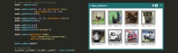
The reinforcement learning agent learns only from visual input, and has access to only the same information given to human players. From a single image the RL agent can learn about the current positions of game objects, but by combining the current image with a few that preceded it, the deep neural network is able to learn not only positions, but also the game’s physical characteristics, such as speed at which objects are moving.
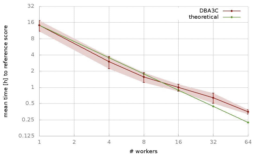
The results of the parallelization experiment conducted by deepesense.ai were impressive – the algorithm required only 20 minutes to master Atari video games, a vast improvement over the approximately one week required in the original experiments done by DeepMind. We provided the code and technical details on arXiv, GitHub and in a blog post, so that others can easily recreate the results. Similar experiments optimizing the training time of Atari games have been conducted by Adam Stooke and Pieter Abbeel from UC Berkeley among others, including OpenAI and Uber.

Replacing the silicon spine

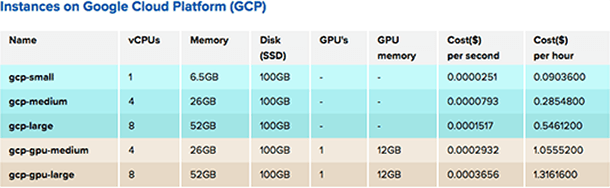
To make the learning process more effective, we used an innovative multi-node infrastructure based on Xeon processors provided by Intel.
The experiment proves that effective machine learning is possible on various architectures, including more common CPUs. The freedom to choose the infrastructure is crucial in seeking ways to further optimize the metrics chosen. Sometimes the time of training is sometimes the decisive factor, at others it is the price of computing power that is the most critical factor. Instead of insisting that all machine learning be done using a particular type of hardware, in practicea diversified architecture may prove more efficient. As machine learning is computing-power-hungry, the wise use of resources may save both money and time.

Biases of mortality revealed by reinforcement learning

Reinforcement learning is much more than just an academic game. By enabling a computer to learn “by itself” with no hints and suggestions,the machine can act innovatively and overcome universal, human biases.
A good example is playing chess. Reinforcement learning agents tend to move in a non-orthodox way that is rarely seen among human players. Sacrificing a bishop only to open the opponent’s position is one of the best examples of superhuman tactics.

So why Atari games?

A typical Atari game provides an environment consisting of a single screen with a limited context and a relatively simple goal to achieve. However, the number of variables which AI must consider is comparable to other visual training environments. Achieving superhuman performance in Atari games is a good indicator that an algorithm will perform well in other tasks. A robotic “game” may mean delivering a human to a destination point without incident or accident or reducing power usage in an intelligent building without any interruption to the business being conducted inside. The huge potential of reinforcement learning is seen in robotics, an area deepsense.ai is continuously developing. Our “Hierarchical Reinforcement Learning with Parameters” paper was presented during the Conference on Robot Learning in 2017 (see a video of a model trained to grab a can of coke below).

A robotic arm can be effectively programmed to perform repetitive tasks like putting in screws on an assembly line. The task is always done in the same conditions, with no variables or unexpected events. But when empowered with reinforcement learning and computer vision, the arm will be able to find a bottle of milk in a refrigerator, a particular book on a bookshelf or a plate in a dryer. The possibilities are practically endless. An interesting demonstration of reinforcement learning in robotics may be seen in the video below, which was taken during an experiment conducted by Chelsea Finn, Sergey Levine and Pieter Abbeel from Cal-Berkeley.

Coding every possible position of milk in every possible fridge would be a Herculean-and unnecessary-undertaking. A better approach is to provide the machine with many visual examples from which it learns features of a bottle of milk and then learns through trial and error how to grasp the bottle. Powered by machine learning, the machine would become a semi-autonomous assistant for elderly or injured people. It would be able to work in different lighting conditions or deal with messy fridges.
Warsaw University professors and deepsense.ai contributors Piotr Miłoś, Błażej Osiński and Henryk Michalewski recently conducted a project dubbed “Learning to Run”. They focused on building software for modern, sophisticated leg prostheses that automatically adjust to the wearer’s walking style. Their model can be easily applied in highly flexible environments involving many rapidly changing variables, like financial markets, urban traffic management or any real-time challenge requiring rapid decision-making.Given the rapid development of reinforcement learning methods, we can be sure that 2018 will bring the next spectacular success in this area.

Spot the flaw – visual quality control in manufacturing

April 19, 2018/in Data science, Deep learning, Machine learning /by Konrad Budek

Quality assurance in manufacturing is demanding and expensive, yes, but also absolutely crucial. After all, selling flawed goods results in returns and disappointed customers. Harnessing the power of image recognition and deep learning may significantly reduce the cost of visual quality control while also boosting overall process efficiency.

According to “Forbes”, automating quality testing with machine learning can increase defect detection rates by up to 90%. Machines never tire, nor lose focus or need a break. And every product on a production line is inspected with the same focus and meticulousness.
Yield losses, the products that need to be reworked due to defects, may be one of the biggest cost-drivers in the production process. In semiconductor production, testing cost and yield losses can constitute up to 30% of total production costs.

Time and money for quality

Traditional quality control is time-consuming. It is manually performed by specialists testing the products for flaws. Yet the process is crucial for business, as product quality is the pillar a brand will stand on. It is also expensive. Electronics industry giant Flex claims that for every 1 dollar it spends creating a product, it lays out 100 more on resolving quality issues.
Since the inception of image recognition software, manufacturers have been able to incorporate IP cameras into the quality control process. Most of the implementations are based on complex systems of triggers. But with the conditions predefined by programmers, the cameras were able to spot only a limited number of flaws. While the technology may not yet have been worthy of the title game changer, the image recognition revolution was one step further.

Deep learning about perfection

Artificial intelligence may enhance the company’s ability to spot flawed products. Instead of embedding complex and lengthy lists of possible flaws into an algorithm, the algorithm learns the product’s features. With the vision of the perfect product, the software can easily spot imperfect ones.

Visual quality control in Fujitsu

A great example of how AI combined with vision systems can improve product quality is on display at Fujitsu’s Oyama factory. The Image Recognition System the company uses not only helps it ensure the production of parts of an optimal quality, but also supervises the assembly process. This dual role has markedly boosted the company’s efficiency.
As the company stated, the solution lacked the flexibility today’s fast-moving world demands. But powering up an AI-driven solution allowed it to quickly adapt its software to new products without the need for time-consuming recalibration. With the AI solutions, Fujitsu reduced its development time by 80% while keeping part recognition rates at 97%+.
As their solution proved successful, Fujitsu deployed it at all of its production sites.
Visual quality control is also factoring in the agricultural product packing arena. One company has recently introduced a high-performance fruit sorting machine that uses computer vision and machine learning to classify skin defects. The operator can teach the sorting platform to distinguish between different types of blemishes and sort the fruit into sophisticated pack grades. The solution combines hardware, software and operational optimization to reduce the complexity of the sorting process.

Summary

As automation becomes more widespread and manufacturing more complex, factories will need to employ AI. Self-learning machines ultimately allow the companies forward-thinking enough to use them to reduce operational costs while maintaining the highest quality possible.
However, an out-of-box solution is not always the best option. Limited flexibility and lower accuracy are the most significant obstacles most companies face. Sometimes building an in-house team of machine learning experts is the best way to provide both the competence and ability to tailor the right solutions for one’s business. As building the internal team to design visual quality control is more than challenging, finding the reliable partner to gain knowledge may be the best option.

Artificial intelligence imagining and reasoning about the future

March 9, 2018/in Data science, Deep learning, Machine learning /by Anna Kowalczyk

Researchers from the deepsense.ai machine learning team, Piotr Miłoś, Błażej Osiński and Henryk Michalewski, together with Łukasz Kaiser from Google Brain’s TensorFlow team optimized infrastructure for reinforcement learning in the Tensor2Tensor project.

The team enhanced an advanced reinforcement learning package with improvements related to the state-of-the-art algorithm called Proximal Policy Optimization, which was originally developed by OpenAI. The algorithm proved to be very versatile and was used to solve games such as Dota 2, robotic tasks like Learning to Run (with our model in sixth place) and Atari games.

AI imagination and reasoning

The idea behind the improvements was to develop an artificial intelligence capable of imagining and reasoning about the future. Instead of using precise and costly simulators or even more costly real-world data, the new AI spends most of its energy on imagining possible future events. The process of imagining is much less costly than gathering real data. At the same time, a properly trained imagination is a far cry from daydreaming. In fact, it makes it possible to precisely model reality and reason about it hundreds of times faster than would be possible using simulators.
The novelty of Tensor2Tensor consists in implementation of the Proximal Policy Optimization, which is completely contained in the computation graph. This is the main technical factor behind the lightning fast imagination.

End-to-end training inside a computation graph

In the second stage of the project the researchers from deepsense.ai, the University of Warsaw and Google Brain are focusing on the end-to-end training of an reinforcement learning agent fully inside a computation graph.

One of the steps in the experiment is the implementation of the Proximal Policy Optimization algorithm entirely using TensorFlow atoms. The training will be run on Cloud Tensor Processing Units (TPUs), which are custom Google-designed chips for machine learning. Assuming that a game simulator can be represented as a neural network, we expect that the whole training process can then be kept in the memory of the Cloud TPU.
Stay tuned for the results of our project!

Starting deep learning hands-on: image classification on CIFAR-10

November 20, 2017/in Deep learning, Neptune /by Piotr Migdal

So, you want to start practicing deep learning? I wrote Learning Deep Learning with Keras as a general overview for using neural networks for image classification. It got quite popular. Yet, I think it is missing one crucial element – practical, hands-on exercises. This post tries to bridge that gap.

Practical deep learning

Deep learning has one dirty secret – regardless how much you know, there is always a lot of trial-and-error. You need to test various network architectures, data preprocessing approaches, parameter and optimizers and so on. Even the top deep learning experts cannot just write a neural network, run it and call it a day.
Each time you see a state-of-the-art neural network and ask yourself “why are there 6 convolutional layers?” or “why do they set dropout rate to 0.3?” the answer is they tried various parameters and chose the ones they did on an empirical basis. However, knowledge of other solutions does give us a good starting point. Theoretical knowledge builds an intuition of which ideas are worth trying and which are unlikely to improve a neural network.
A fairly general approach to solving any deep learning problem is:

use some state-of-the-art architecture for a given class of problems,
modify it to optimize performance for your particular problem.

Modification goes both with changing its architecture (e.g. the number of layers, adding or removing auxiliary layers like dropout or batch normalization) and tuning its parameters. The only performance measure that matters is the validation score, i.e. if a network trained on one dataset is able to make good predictions on a new one it has never encountered. Everything else boils down to experimentation and tweaking.

deepsense.ai Kaggle Leaderboard for Right Whale Recognition

Kaggle Leaderboard for the Right Whale Recognition competition

I like bringing the example of Right Whale Recognition – a Kaggle competition which our deepsense.ai team won by a large margin. All top teams used convolutional neural networks. I was surprised to see that other winners used very similar architectures (clearly, it was a starting point without which it would be hard to accomplish a lot). The many, many small optimizations we made made a huge difference in the performance of our network.

A good dataset – CIFAR-10 for image classification

Many introductions to image classification with deep learning start with MNIST, a standard dataset of handwritten digits. This is unfortunate. Not only does it not produce a “Wow!” effect or show where deep learning shines, but it also can be solved with shallow machine learning techniques. In this case, plain k-Nearest Neighbors produces more than 97% accuracy (or even 99.5% with some data preprocessing!). Moreover, MNIST is not a typical image dataset – and mastering it is unlikely to teach you transferable skills that would be useful for other classification problems.

“Many good ideas will not work well on MNIST (e.g. batch norm). Inversely[,] many bad ideas may work on MNIST and no[t] transfer to real [computer vision]” – a tweet by François Chollet (creator of Keras).

If you really need to stick with a 28×28 grayscale image dataset, there is notMNIST (A-J letters from strange fonts) and a MNIST-like dataset with fashion products. They are slightly better, and harder. However, I think that there is no excuse for avoiding using actual photos.
We will work on CIFAR-10, a classic dataset of small color images. It has 60k of 32×32 pixel images, each belonging to one of ten classes. 50k are in the training set (i.e. the one we use to train our neural network) and 10k are in the validation dataset. Have a look at these sample pictures:

CIFAR-10 classes with example images

Getting our hands dirty

I really encourage you to do the exercises. Sure, it is much faster to just read. But with data science (and programming in general) it matters more how much you write than read. After all, if you want to learn to swim you won’t master it unless you actually dip your toes in the water.
Before we get started:

Create a Neptune account (we give you $5 for computing, so no worries – this tutorial won’t cost you a cent; you’re not likely to use up more than $5 worth of your credit).
Clone or copy the repository https://github.com/deepsense-ai/hands-on-deep-learning/ – all scripts we use need to be run from its cifar_image_classification directory.
On Neptune, click on projects and create a new one – CIFAR-10 (with code: CIF).

The code is in Keras, a high-level Python neural network library. We will use Python 3 and TensorFlow backend. The only Neptune-specific part of this code is logging. If you want to run it on another infrastructure, just change a few lines.

Architectures and blocks (in Keras)

One thing that differentiates deep learning from classical machine learning is its compositional architecture. Instead of using a one-step classifier (be it Logistic Regression, Random Forest or XGBoost) we create a network out of blocks (called layers).

Deep Learning metaphors: ConvNet layers as Jenga blocks

Logistic regression

Let’s start with something simple – a multi-class logistic regression. It is a “shallow” machine learning technique, yet can be expressed in the language of neural networks. Its architecture consists of only one meaningful layer. In Keras, we write the following:

model = Sequential()
model.add(Flatten(input_shape=(32, 32, 3)))
model.add(Dense(10))
model.add(Activation('softmax'))
model.compile(optimizer=’adam’,
              loss='categorical_crossentropy',
              metrics=['accuracy'])

If we want to see step-by-step what happens with our data flow, with respect to dimensions and the number of weights to be optimized, we can use my keras-sequential-ascii script:

           OPERATION           DATA DIMENSIONS   WEIGHTS(N)   WEIGHTS(%)
               Input   #####     32   32    3
             Flatten   ||||| -------------------         0      0.0%
                       #####        3072
               Dense   XXXXX -------------------     30730    100.0%
             softmax   #####          10

The flatten layer just transforms (x, y, channels) into a flat vector of pixel values. The dense layer connects all inputs to all outputs. Softmax then changes real numbers into probabilities.
To run it, just type in the terminal:

$ neptune send lr.py

This opens a browser tab in which you can keep track of the training process. You can even look up misclassified images. However, this linear model will look mostly for colors and their locations on the image.

Neptune channels dashboard showing misclassified images

The overall score is not impressive. I got 41% accuracy on the training set and, more importantly, 37% on validation. Note that 10% is a baseline for making random guesses.

Multilayer perceptron

Old-school neural networks consist of a few dense layers. Between the layers we need to use an activation function. This function, applied on each component separately, allows us to make it non-linear, capturing much more complex patterns than logistic regression does. The historical approach (motivated by an abstraction of biological neural networks) is to use a sigmoid.

model = Sequential()
model.add(Flatten(input_shape=(32, 32, 3)))
model.add(Dense(128, activation='sigmoid'))
model.add(Dense(128, activation='sigmoid'))
model.add(Dense(10))
model.add(Activation('softmax'))
model.compile(optimizer=adam,
             loss='categorical_crossentropy',
             metrics=['accuracy'])

What does this mean for our data?

          OPERATION           DATA DIMENSIONS   WEIGHTS(N)   WEIGHTS(%)
              Input   #####     32   32    3
            Flatten   ||||| -------------------         0     0.0%
                      #####        3072
              Dense   XXXXX -------------------    393344    95.7%
            sigmoid   #####         128
              Dense   XXXXX -------------------     16512     4.0%
            sigmoid   #####         128
              Dense   XXXXX -------------------      1290     0.3%
            softmax   #####          10

We used two additional (so-called hidden) layers, each with with sigmoid as its activation function. Let’s run it!

$ neptune send mlp.py

I suggest creating a custom chart combining both training and validation channels on one plot.

Accuracy and log-loss for training and validation sets, live

In principle, even with a single hidden layer it is possible to approximate any function (see the universal approximation theorem). However, that does not yet mean that it works well in practice, with a finite amount of data. If the hidden layer is too small, it is not able to approximate any function. When it gets too big, the network can easily overfit – i.e. memorize training data, but not be generalizable to other images. Any time your training score goes up at the cost of the validation score, your network overfits.
We can get to around 45% accuracy on the validation set, which is an improvement over logistic regression. Yet we can easily do much better. If you want to play with this kind of network – edit file, run it (I suggest adding –tags my-experiment) in the command line and see if you can do better. Make a few approaches, and see how it goes.
Hints:

Use more than 20 epochs.
In practice, neural networks use 2-3 dense layers.
Make big changes to see a difference. In this case change the hidden layer size by 2x or even 10x.

Just because you should in theory be able to create any picture (or even any photograph) with MS Paint, drawing pixel-by-pixel, it does not mean it will work in practice. We need to take advantage of the spatial structure and use a convolutional neural network (often abbreviated as ConvNet or CNN).

Convolutional neural networks

Instead of trying to connect everything with everything, we can process images in a smarter way. Convolution is an operation which performs the same local operation on each part of the image. Some examples of what convolution can do include blurring, amplifying edges or detecting color gradients – see Image Kernels – Visually Explained.
Each convolution layer produces new channels based on those which preceded it. First, we start with 3 channels for red, green and blue (RGB) components. Next, channels get more and more abstract. To get some idea of what is going on, visit How neural networks build up their understanding of images to see patterns that activate subsequent layers – from simple colors and gradients to much more complex patterns.
As we create channels representing various properties of the image, we need to reduce the resolution (usually with max-pooling). Also, modern networks typically use ReLU as the activation function as it works much better for deeper models.

model = Sequential()
model.add(Conv2D(32, (3, 3), activation='relu',
                 input_shape=(32, 32, 3)))
model.add(MaxPool2D())
model.add(Conv2D(64, (3, 3), activation='relu'))
model.add(MaxPool2D())
model.add(Flatten())
model.add(Dense(10))
model.add(Activation('softmax'))
model.compile(optimizer='adam',
              loss='categorical_crossentropy',
              metrics=['accuracy'])

Network architecture looks like this:

          OPERATION           DATA DIMENSIONS   WEIGHTS(N)   WEIGHTS(%)
              Input   #####     32   32    3
             Conv2D    |/  -------------------       896     2.1%
               relu   #####     30   30   32
       MaxPooling2D   Y max -------------------         0     0.0%
                      #####     15   15   32
             Conv2D    |/  -------------------     18496    43.6%
               relu   #####     13   13   64
       MaxPooling2D   Y max -------------------         0     0.0%
                      #####      6    6   64
            Flatten   ||||| -------------------         0     0.0%
                      #####        2304
              Dense   XXXXX -------------------     23050    54.3%
            softmax   #####          10

To run it, we type:

$ neptune send cnn_simple.py

Even with this simple neural network we get 70% accuracy on validation. That is much more than we got with logistic regression or a multilayer perceptron!
Now, feel free to experiment.
Hints:

Play with the number of channels and how they grow.
Usually 3×3 convolutions work the best; stick to them (and 1×1 convolutions which only mix channels).
You can have 1-3 convolutional layers before each MaxPool operation.
Adding a Dense layer may help.
Between dense layers you can use Dropout, to reduce overfitting (i.e. if you see that training accuracy is higher than validation accuracy).

So, is that it? No! This is only the beginning.
To compare results, click on the project name. You will see the whole list of projects. In Manage columns, tick all accuracy (and possible log-loss) scores. You can order your results using validation accuracy. You get some sort of your own personal Kaggle leaderboard!

Your personal, configurable Kaggle Leaderboard

In addition to architecture (which is a big deal), optimizers significantly change the accuracy of the overall results. Very often, we get better results by adding more epochs (i.e. the number of times the whole training dataset is processed) and reducing the learning rate at the same time.
For example, try this network I wrote:

          OPERATION           DATA DIMENSIONS   WEIGHTS(N)   WEIGHTS(%)
              Input   #####     32   32    3
             Conv2D    |/  -------------------       896     0.1%
               relu   #####     32   32   32
             Conv2D    |/  -------------------      1056     0.2%
               relu   #####     32   32   32
       MaxPooling2D   Y max -------------------         0     0.0%
                      #####     16   16   32
 BatchNormalization    μ|σ  -------------------       128     0.0%
                      #####     16   16   32
            Dropout    | || -------------------         0     0.0%
                      #####     16   16   32
             Conv2D    |/  -------------------     18496     2.9%
               relu   #####     16   16   64
             Conv2D    |/  -------------------      4160     0.6%
               relu   #####     16   16   64
       MaxPooling2D   Y max -------------------         0     0.0%
                      #####      8    8   64
 BatchNormalization    μ|σ  -------------------       256     0.0%
                      #####      8    8   64
            Dropout    | || -------------------         0     0.0%
                      #####      8    8   64
             Conv2D    |/  -------------------     73856    11.5%
               relu   #####      8    8  128
             Conv2D    |/  -------------------     16512     2.6%
               relu   #####      8    8  128
       MaxPooling2D   Y max -------------------         0     0.0%
                      #####      4    4  128
 BatchNormalization    μ|σ  -------------------       512     0.1%
                      #####      4    4  128
            Dropout    | || -------------------         0     0.0%
                      #####      4    4  128
            Flatten   ||||| -------------------         0     0.0%
                      #####        2048
              Dense   XXXXX -------------------    524544    81.6%
               relu   #####         256
            Dropout    | || -------------------         0     0.0%
                      #####         256
              Dense   XXXXX -------------------      2570     0.4%
            softmax   #####          10

$ neptune send cnn_adv.py

It will take around 0.5h, but the results will be much better. Patience pays off – validation accuracy should be around 83%!
You can try other examples of networks for CIFAR-10: one from the Keras repository (though I had trouble reproducing their score) and one from this blog post. Both of them train in around 1.5h.

$ neptune send cnn_fchollet.py
$ neptune send cnn_pkaur.py

Can you do better? :)
Maybe you can beat 83%? Or create a network which achieves the same goal, but is much simpler? Or one that trains much faster? If you do better, I encourage you to post your validation score in the comments below, with a link to network architecture (e.g. via a link to your GitHub repo or a gist).

Image classification sample solution for Kaggle competition

October 24, 2017/in Deep learning, Neptune /by Jakub Czakon

At deepsense.ai, we’re doing our best to make our mark in state‑of‑the‑art data science. For many years, we have been competing in machine learning challenges, gaining both conceptual and technical expertise. Now, we have decided to open source an end‑to‑end image classification sample solution for the ongoing Cdiscount Kaggle competition. In so doing, we believe we’ll encourage data scientists both seasoned and new to compete on Kaggle and test their neural nets.

Introduction

Competing in machine learning challenges is fun, but also a lot of work. Participants must design and implement end‑to‑end solutions, test neural architectures and run dozens of experiments to train deep models properly. But this is only a small part of the story. Strong Kaggle competition solutions have advanced data pre‑ and post‑processing, ensembling and validation routines, to name just a few. At this point, competing effectively becomes really complex and difficult to manage, which may discourage some data scientists from rolling up their sleeves and jumping in. Here at deepsense.ai we believe that Kaggle is a great platform for advanced data scientific training at any level of expertise. So great, in fact, that we felt compelled to open‑source an image classification sample solution to the currently open Cdiscount challenge. Below, we describe what we have prepared.

Image classification sample solution overview

When we say our solution is end‑to‑end, we mean that we started with raw input data downloaded directly from the Kaggle site (in the bson format) and finish with a ready‑to‑upload submit file. Here are the components:

data loader
1. Keras custom iterator for bson file
2. label encoder representing product IDs to fit the Keras API
neural network training on n classes and k examples per class. We use the following architectures:
1. MobileNet (Howard et al. ’17)
2. Inception v3
3. ensembles of the models mentioned above
model predictions
1. single-model prediction
2. ensembling (by averaging) for multiple models
submit generation

For instance, the image classification with MobileNets ensemble would be defined as followings:

@register_pipeline
def MobilenetEnsemblePipeline(num_classes, epochs, workers, models_dir):
	pipe_legs_params = {'mobilenet_128_{}'.format(num_classes): (128, 128),
	                    'mobilenet_160_{}'.format(num_classes): (160, 64),
	                    'mobilenet_192_{}'.format(num_classes): (192, 32),
	                    }
	pipe_legs = []
	for name, (target_size, batch_size) in pipe_legs_params.items():
		leg = DeepPipeline([('loader', KerasDataLoader(num_classes, target_size, batch_size)),
		                    ('model', KerasMobileNet(
			                    architecture_cfg={'input_size': target_size, 'classes': num_classes},
			                    training_cfg={'epochs': epochs, 'workers': workers, 'verbose': 1},
			                    callbacks_cfg={'models_dir': models_dir, 'model_name': name}))])
		pipe_legs.append((name, leg))
	pipe_avg = PredictionAverage(pipe_legs)
	pipeline = LabelEncoderWrapper(pipe_avg)
	return pipeline

Watch this video for quick code overview:

What if I want to use my network architecture?

You are encouraged to replace our network with your own. Below you can find a short snippet of code that you simply place in the models.py file:

class MyModel(BasicKerasClassifier):
    def _build_model(self, params):
        return Model

Otherwise I would suggest extending BasicKerasClassifier, or KerasDataLoader with custom augmentations, learning rate schedules and other tricks of your choice.

How to get started?

To start using our pipeline, follow these steps:

download the source code from https://github.com/deepsense-ai/cdiscount-starter
follow the README instructions to run the code
modify this image classification sample solution to fit your needs
have fun competing on Kaggle!

Image classification sample solution - neptune dashboard with Kaggle experiment

Image classification sample solution running in Neptune. Live charts presents log-loss and accuracy for the running experiment.

Final remarks

Feel free to use, modify and run this code for your own purposes. We run multiple of them on Neptune, which you may find useful for managing your experiments.

Logo detection and brand visibility analytics – example

August 29, 2019/in Data science, Deep learning, Machine learning, Neptune /by Michal Romaniuk and Konrad Budek

Companies pay astonishing amounts of money to sponsor events and raise brand visibility. Calculating the ROI from such sponsorship can be augmented with machine learning-powered tools to deliver more accurate results.

Event sponsoring is a well-established marketing strategy to build brand awareness. Despite being one of the most recognizable brands in the automotive industry, Chevrolet pays $71.4 million dollars each year to put its brand on Manchester United shirts.

How many people does your brand reach?

According to Eventmarketer’s study, 72% of consumers positively view brands that provide them with positive experiences, be it a great sports game or another cultural event, such as a music festival. Such events attract large numbers of viewers both directly and via media reports, allowing brands to get favorable positioning and work on their word-of-mouth recognition.

Sponsorship contracts often come at a steep price, so brand owners are naturally more than a little interested in finding out how effectively their outlays are working for them. However, it’s difficult to assess quantitatively just how great the brand exposure is in a given campaign. The information on brand exposure can further support demand forecasting efforts, as the company gains information on expected demand peaks that result from greater brand exposure in media coverage.

The current approach to computing such statistics has involved manually annotating broadcast material, which is tedious and expensive. To address these problems, we have developed an automated tool for logo detection and visibility analysis that provides both raw detection and a rich set of statistics.

Solution overview

We decided to break the problem down into two steps: logo detection with convolutional neural networks and an analytics for computing summary statistics.

The main advantage of this approach is that swapping the analytics module for a different one is straightforward. This is essential when different types of statistics are called for, or even if the neural net is to be trained for a completely different task (we had plenty of fun modifying this system to spot and count coins – stay tuned for a future blog post on that).

Logo detection with deep learning

There are two principal approaches to object detection with convolutional neural networks: region-based methods and fully convolutional methods.

Region-based methods, such as R-CNN and its descendants, first identify image regions which are likely to contain objects (region proposals). They then extract these regions and process them individually with an image classifier. This process tends to be quite slow, but can be sped up to some extent with Fast R-CNN, where the image is processed by the convolutional network as a whole and then region representations are extracted from high-level feature maps. Faster R-CNN is a further improvement where region proposals are also computed from high-level CNN features, which accelerates the region proposal step.

Fully convolutional methods, such as SSD, do away with processing individual region proposals and instead aim to output class labels where the region proposal step would be. This approach can be much faster, since there is no need to extract and process region proposals individually. In order to make this work for objects with very different sizes, the SSD network has several detection layers attached to feature maps of different resolutions.

Since real-time video processing is one of the requirements of our system, we decided to go with the SSD method rather than Fast R-CNN. Our network also uses ResNet-50 as its convnet backbone, rather than the default VGG-16. This made it much less memory-hungry, while also helping to stabilize the training process.

Model training

In the process of refining the SSD architecture for our requirements, we ran dozens of experiments. This was an iterative process with a large delay between the start and finish of an experiment (typically 1-2 days). In order to run numerous experiments in parallel, we used Neptune, our machine learning experiment manager. Neptune captures the values of the loss function and other statistics while an experiment is running, displaying them in a friendly web UI. Additionally, it can capture images via image channels and display them, which really helped us troubleshoot the different variations of the data augmentation we tested.

Logo detection analytics

The model we produced generates detections very well. However, when even a short video is analyzed, the raw description can span thousands of lines. To help humans analyze the results, we created software that translates these descriptions into a series of statistics, charts, rankings and visualizations that can be assembled into a concise report.

The statistics are calculated globally and per brand. Some of them, like brand display time, are meant to be displayed, but many are there to fuel the visual representation. Speaking of which, the charts are really expressive in this task. Some features include brand exposure size in time, heatmaps of a logo’s position on the screen and bar charts to allow you to easily compare various statistics across the brands. Last but not least, we have a module for creating highlights – visualizations of the bounding boxes detected by the model. This module serves a double purpose: in addition to making the analysis easy to track, such visualizations are also a source of valuable information for data scientists tweaking the model.

Results

We processed a short video featuring a competition between rivals Coca-Cola and Pepsi to see which brand received more exposure in quantitative terms. You can watch it on YouTube by following this link. Which logo has better visibility?

Below, you can compare your guesses with what our model reported:

Possible extensions

There are many business problems where object detection can be helpful. Here at deepsense.ai, we have worked on a number of them.

We developed a solution for Nielsen that extracts information about ingredients from photographs of FMCG products, using object detection networks to locate the list of ingredients in photographs of products. This made Nielsen’s data collection more efficient and automatic. In its bid to save the gravely endangered North Atlantic Right Whale,The NOAA used a related technique to spot whales in aerial photographs. Similar techniques are used when the reinforcement learning-based models behind autonomous vehicles learn to recognize road signs.

With logo detection technology, companies can evaluate a campaign’s ROI by analyzing any media coverage of a sponsored event. With the information on brand positioning in hand, it is easy to calculate the advertising equivalent value or determine the most impactful events to sponsor.

With further extrapolation, companies can monitor the context of media coverage and track whether their brand is shown with positive or negative information, providing even more knowledge for the marketing team.

Using deep learning for Single Image Super Resolution

October 23, 2017/in Data science, Deep learning /by Katarzyna Kańska

Single Image Super Resolution involves increasing the size of a small image while keeping the attendant drop in quality to a minimum. The task has numerous applications, including in satellite and aerial imaging analysis, medical image processing, compressed image/video enhancement and many more. In this blog post we apply three deep learning models to this problem and discuss their limitations and promising ways to overcome them.

Single Image Super Resolution: Problem statement

Our objective is to take a low resolution image and produce an estimate of a corresponding high‑resolution image. This problem is ill‑posed – multiple high‑resolution images can be produced from the same low‑resolution image. For instance, suppose we have a 2×2 pixel sub‑image containing a small vertical or horizontal bar [Fig. 1]. Regardless of the orientation of the bar, these 4 pixels will correspond to just one pixel in a picture downscaled 4 times. With real life images, one needs to overcome an abundance of similar problems, making the task difficult to solve.

First, let’s introduce a quantitative quality‑measurement method to evaluate and compare the models. For each model implemented, we will compute a metric commonly used to measure the quality of reconstruction of lossy compression codecs, called Peak Signal to Noise Ratio (PSNR). This metric is a de‑facto standard used in Super Resolution research. It measures how much the distorted image (possibly of lower quality) deviates from the original high‑quality image. In this setting, PSNR is the ratio of maximum possible pixel value of the image (signal strength) to maximum mean squared error (MSE) between the original image and its estimated version (noise strength), expressed in logarithmic scale.

$PSNR = 10 cdot log_{10}frac{MAX_I^2}{MSE}$

The larger the PSNR values, the better the reconstruction, and therefore maximization of PSNR naturally leads to minimizing MSE as the objective function. That was our approach in two out of three models we present here.
In our experiments, we trained the models to upscale input images four times (in terms of width and height). Above this factor, upscaling even small images becomes hard – for example, an image upscaled eight times has a 64x bigger pixel count. Storing it consequently requires 64x more memory in raw form, to which it is converted during training.
We have tested our models on benchmarks commonly used in the literature – Set5, Set14 and BSD100. The performance of the models described on these datasets is cited in the papers, which allowed us to compare our results to those other authors have put forward.
The models were implemented in PyTorch, an open‑source neural network framework developed by Facebook.

Why deep learning?

One of the most commonly used techniques for upscaling an image is interpolation. Although simple to implement, this method leaves much to be desired in terms of visual quality, as the details (e.g. sharp edges) are often not preserved.

**Figure 2:** Most common interpolation methods produce blurry images. From top to bottom:
nearest neighbour interpolation, bilinear interpolation and bicubic interpolation. The image
was upscaled 4x.

More sophisticated methods exploit internal similarities of a given image or use datasets of low‑resolution images and their high‑resolution counterparts, effectively learning a mapping between them. Among example‑based SR algorithms, the sparse‑coding‑based method is one of the most popular.
This method requires a dictionary to be found that will allow us to map low resolution images into an intermediate, sparse representation. In addition, the HR dictionary is learned, and will allow us to restore our estimate of a high resolution image. Such a pipeline usually involves several steps and not all of them can be optimized. Ideally we would like to have all of these steps combined in one big step with all of its parts being optimizable. That effect can be achieved by a neural network, the architecture of which is inspired by sparse coding.
See more here.

SRCNN

SRCNN was the first deep learning method to outperform traditional ones. It is a convolutional neural network consisting of only 3 convolutional layers: patch extraction and representation, non‑linear mapping and reconstruction.
Before being fed into the network, an image needs to be upsampled via bicubic interpolation. It’s then converted to YCbCr color space, while only luminance channel (Y) is used by the network. The network’s output is then merged with interpolated CbCr channels to produce a final color image. We chose this procedure because we are not interested in changing colors (this is the information stored in the CbCr channels), but only their brightness (the Y channel), and ultimately because human vision is more sensitive to luminance (“black and white”) differences than chromatic differences.
We found SRCNN really difficult to train. It was sensitive to hyperparameter changes, and the set‑up presented in the paper (learning rate 10^-4 for the first two layers, 10^-5 for the last layer, SGD optimizer) caused our PyTorch implementation to produce sub‑optimal results. We observed small changes under some different learning rates, but in the end the thing that gave us the biggest performance boost was switching to Adam optimizer, with a learning rate of 10^-5 used for all layers. The final network was trained on 14k 32×32 subimages from the same dataset as in original paper (91 images).

Perceptual loss

Although SRCNN is already better than standard methods, there are some ways in which it can still be enhanced. As mentioned earlier, the network is unstable, and one may also wonder whether optimizing MSE is an optimal choice.
Clearly, the images obtained by minimizing MSE are overly smooth. (MSE tends to produce an image resembling the mean of all possible high resolution pictures, resulting in a given low resolution picture [Fig. 1]). MSE also does not capture the perceptual differences between the model’s output and the ground truth image. Consider a pair of images, where the second one is a copy of the first, but shifted a few pixels to the left. For a human the copy looks almost indistinguishable from the original, but even such a small change can cause PSNR to decrease dramatically.
How should the perceived content of a given image be preserved? A similar arises in neural style transfer, and perceptual loss is a potential solution. It too optimizes MSE, but instead of using the model output itself, one can use the high‑level image feature representations extracted from pretrained convolutional neural networks (in our case output from 7th layer of VGG16). The intuition behind this idea is that a network trained for image classification (like VGG) stores in its feature maps the information on what details of common objects look like. And we want our upscaled image to be made up of objects resembling real world ones as much as possible.
Apart from changing the loss function, network architecture is also remodeled. The model is much deeper than SRCNN, uses residual blocks and does most of the processing on low‑resolution images (which accelerates training and inference). Upscaling also happens inside the network. In their paper, the authors used transposed convolutions (also called deconvolutions) with kernel 3×3 and stride=2 for that purpose. Artifacts produced by this model seemed similar to those known as the checkerboard effect. To reduce this effect we also tried deconvolution with a 4×4 kernel and nearest neighbor interpolation followed by a 3×3 convolutional layer with stride=1. In the end, interpolation followed by convolutional layer gave the best results, but didn’t remove the artifacts completely. Similar effects were observed in the original report.
Similar to the process described in paper, our training pipeline consisted of a dataset of 288×288 random crops from nearly 10k images from MS‑COCO. We set the learning rate to 10^-3 and used Adam as our optimizer. Unlike in the paper cited above, we skipped post‑processing (histogram matching) as it didn’t provide any improvement.

SRResNet

In order to maximise our PSNR performance, we decided to implement a network called SRResNet, which achieves state‑of‑the‑art results on standard benchmarks. The original paper mentions a way of extending it in a way that allows more high frequency details to be restored.
As with the residual network described in the previous paragraph, SRResNet’s residual blocks architecture is based on this post. There are two minor additions: first, SRResNet uses Parametric ReLU instead of ReLU, which generalizes the former by introducing a learnable parameter that makes it possible to adaptively learn the negative part coefficient. The other difference is the image upsampling method used – in SRResNet, sub‑pixel convolutional layers are used. This technique is thoroughly explained here.
The images generated by the SRResNet we trained are almost indistinguishable from the results presented in the paper. The training took two days, during which we used Adam optimizer with a learning rate of 10^-4. The dataset used consisted of 96×96 random crops from MS‑COCO, similar to the perceptual loss network.

Future work

There are several promising deep learning‑based approaches to single image super resolution that we didn’t test due to time constraints.
This recent paper mentions superb PSNR results gained thanks to the use of a modified SRResNet architecture. The authors remove batch normalization from the residual layers, and increase the number of residual layers used from 16 to 32. The resulting network trains for seven days on NVIDIA Titan Xs. Our implementation of SRResNet trained for two days to get our results, which allowed for faster iterations and more efficient hyperparameter tuning, but would not be possible had the ideas described been implemented.
Our perceptual loss experiments show that PSNR may not be a good metric to use for evaluating super resolution networks. In our opinion, more research needs to be done on different types of perceptual loss. In the papers we have examined, we’ve only seen simple MSE between VGG feature map representations of network output and ground truth. It’s unclear why MSE, being a per‑pixel loss, would be a good choice in this case.
Another promising direction for super resolution is Generative Adversarial Networks. This original paper extends SRResNet by using it as part of the architecture called SRGAN. Images generated by the resulting network contain high frequency details, like animals’ fur or grass straws. While they may look more believable, the images generated suffer in the PSNR statistics.

**Figure 4:** From top to bottom: the image produced by our SRResNet implementation,
the image produced by SRResNet extension, and the original image

Conclusion

In this blogpost we have described our experiments with three different convolutional neural networks used for Single Image Super Resolution. The table below summarizes our results.

SRCNN	Perceptual loss	SRResNet
+ short inference + better than standard methods – worst results among deep learning approaches	+ more natural looking results than SRCNN – strong artifacts	+ state‑of‑the‑art results – long inference

Figure 5: Advantages and disadvantages of the models discussed

Even a simple three layer SRCNN was able to beat most non‑deep‑learning methods when measured on standard benchmark datasets using PSNR. Our examinations of perceptual loss showed, however, that this measure is not perfect for evaluating our model’s performance, as we were able to produce visually appealing images that were much worse than bicubic interpolation when evaluated with PSNR. Finally, we reimplemented SRResNet and reproduced state‑of‑the‑art results on benchmark datasets.

References

[1] Image Super‑Resolution Using Deep Convolutional Networks
[2] Perceptual Losses for Real‑Time Style Transfer and Super‑Resolution
[3] Photo‑Realistic Single Image Super‑Resolution Using a Generative Adversarial Network
[4] Enhanced Deep Residual Networks for Single Image Super‑Resolution
[5] Real‑Time Single Image and Video Super‑Resolution Using an Efficient Sub‑Pixel Convolutional Neural Network
[6] Training and investigating Residual Nets

Fall 2017 release – launching Neptune 2.1 today!

October 12, 2017/in Data science, Deep learning, Machine learning, Neptune /by Mariusz Gądarowski

We’re thrilled today to announce the latest version of Neptune: Machine Learning Lab. This release will allow data scientists using Neptune to take some giant steps forward. Here we take a quick look at each of them.

Cloud support

One of the biggest differences between Neptune 1.x and 2.x is that 2.x supports Google Cloud Platform. If you want to use NVIDIA® Tesla® K80 GPUs to train your deep learning models or Google’s infrastructure for your computations, you can just select your machine type and easily send your computations to the cloud. Of course, you can still run experiments on your hardware the way it was. We currently support only GCP–but stay tuned as we will not only be bringing more clouds and GPUs into the Neptune support fold, but offering them at even better prices!
With cloud support, we are also changing our approach to managing data. Neptune uses shared storage to store data about each experiment, for both the source code and the results (channel values, logs, output files, e.g. trained models). On top of that, you can upload any data to a project and use it in your experiments. As you execute your experiments, you’ve got all your sources at your fingertips, in the /neptune directory, which is available on fast drive for reading and writing. It is also your current working directory – just like you would run it on your local machine. Alongside this feature, Neptune can still keep your original sources so you can easily reproduce your experiments. For more details please read documentation.

Interactive Notebooks

Engineers love how interactive and easy to use Notebooks are, so it should come as no surprise that they’re among the most frequently used data science tools. Neptune now allows you to prototype faster and more easily using Jupyter Notebooks in the cloud, which is fully integrated with Neptune. You can choose from among many environments with different libraries (Keras, TensorFlow, Pytorch, etc) and Neptune will save your code and outputs automatically.

New Leaderboard

Use Neptune’s new leaderboard to organize data even more easily.
You can change the width of all columns and reorder them by simply drag and dropping their headings.

You can also edit the name, tags and notes directly in the table and display metadata including running time, worker type, environment, git hash, source code size and md5sum.

The experiments are now presented with their Short ID. This allows you to identify an experiment among those with identical names.

Sometimes you may want to see the same type of data throughout the entire project. You can now fix chosen columns on the left for quick reference as you scroll horizontally through the other sections of the table.

Parameters

Neptune comes with new, lightweight and yet more expressive parameters for experiments.
This means you no longer need to define parameters in configuration files. Instead, you just write them in the command line!
Let’s assume you have a script named main.py and you want to have 2 parameters: x=5 and y=foo . You need to pass them in the neptune send command:

neptune send -- '--x 5 --y foo'

Under the hood, Neptune will run python main.py –x 5 –y foo , so your parameters are placed in sys.argv . You can then parse these arguments using the library of your choice.
An example using argparse :

import argparse
parser = argparse.ArgumentParser()
parser.add_argument('--x', type=int)
parser.add_argument('--y')
params = parser.parse_args() # params.x = 5, params.y = 'foo'

If you want Neptune to track a parameter, just write ‘%’ in front of its value — it’s as simple as that!

neptune send -- '--x %5 --y %foo'

The parameters you track will be displayed on the experiment’s dashboard in the UI. You will be able to sort your experiments by parameter values.

The new parameter syntax supports grid search for numeric and string parameters:

neptune send -- '--x %[1, 10, 100] --y %(0.0, 10.0, 0.1)'
neptune send -- '--classifier %["SVM", "Naive Bayes", "Random Forest"]'

You can read more about the new parameters in our documentation.

Try Neptune 2.1

If you still haven’t tried Neptune, give it a go today! Sign up for a free! It takes just 2 minutes to get started! Neptune’s community forum and detailed documentation will help you navigate the process.

Solving Atari games with distributed reinforcement learning

October 4, 2017/in Data science, Deep learning, Neptune /by Igor Adamski

At deepsense.ai, we strive to make our mark on the cutting-edge research leading towards intelligent machines by providing practical machine learning tools and designs that make it much easier for scientists to track their experiments and verify novel ideas.

One particular step towards achieving this ideal was distributing a state-of-the-art Reinforcement Learning algorithm on a large CPU cluster, allowing super-fast training of agents that learned to master a wide range of Atari 2600 games. This post contains a brief description of our Distributed Deep Reinforcement Learning experiments. For a more in-depth look you can read our paper on the matter here.

Distributed reinforcement learning

Atari games are a widely accepted benchmark for deep reinforcement learning (RL). One common characteristic of these games is that they are very easy for humans to crack conceptually. Comparing the time it takes humans and computers to master these games can provide a clear indication of the capabilities of modern artificial intelligence. The first approaches to teach an agent to play Atari were developed by DeepMind and required around a week of training. The A3C algorithm developed later was able to achieve human performance in most games and did so with a similar amount of training time. But could computers ever learn faster than us?
Creating such a quick and bright Atari games learner would mean that computers outpaced us in understanding a game environment. The techniques that said agent would use to quickly develop a good grasp of the game could be studied to further develop our understanding of the cognitive features of a human brain. Moreover, faster training would give researchers considerably more flexibility in terms of experimenting and thus make verifying various RL approaches much quicker. Today, we present a Distributed Reinforcement Learning algorithm that efficiently trains on a large cluster of 64 12-core CPUs (768 cores in total). Our design enables agents to learn to play Atari games in as little as 20 minutes. We’re making our implementation available here.

	Breakout
Initial performance	After 15 minutes of training	After 30 minutes of training

	Assault
Initial performance	After 15 minutes of training	After 30 minutes of training

	Boxing
Initial performance	After 15 minutes of training	After 30 minutes of training

Our achievement and results

By distributing the BA3C (details of single-machine implementation here) reinforcement learning algorithm, we were able to make an agent teach itself to play a wide range of Atari games rapidly, by just looking at a raw pixel output (game screen) from the game emulator. Our best experiments were distributed across 64 machines, each of which had 12 Intel CPU cores. In the game of Breakout, our agent achieves a superhuman score in just 20 minutes, which is a significant reduction of the single machine implementation learning time.
Training for Breakout on a single computer takes around 15 hours, bringing our implementation very close to the theoretical scaling (assuming computational power is maximized, using 64 times more CPUs should yield a 64-fold speed-up). The graph below shows the scaling of our implementation for different numbers of machines. Moreover, our algorithm exhibits robust results on many Atari environments, meaning that it is not only fast, but also adaptable to various learning tasks.

Scaling graph showing the mean time to achieve a good score in Atari's Breakout using our distributed reinforcement learning algorithm

Graph showing the mean time of our algorithm (DBA3C) to achieve a score of 300 in the game of Breakout (average score of 300 needs to be obtained in 50 consecutive tries). The green line shows the theoretical scaling in reference to a single machine implementation.

Using Neptune, a tool developed here at deepsense.ai, we were able to proactively track the performance of our agents. This enabled us to instantly verify if a certain feature of the algorithm works as expected. In Neptune, we could observe our agents’ real-time scores along with many other experiment-related metrics that we later used to optimize the algorithm. The graph below shows training curves from 10 different experiments on the Breakout game. Graphs were updated live in Neptune as the training went on.

Mean score on Atari's Breakout in our distributed reinforcement learning set-up

A plot showing the live mean score obtained by the agent in 50 consecutive trials of Breakout

We managed to achieve very competitive training times. As we hope to inspire further research in the RL domain, we decided to open-source the implementation of our distributed reinforcement learning algorithm.

Details of the implementation

In the following section we describe the technicalities of our distributed set-up, aiming primarily to address a more advanced audience. To get the most out of our description, we recommend readers familiarize with this study done by the Google Brain team.
For parallelization we chose the synchronous paradigm. Synchronizing all our workers yielded much faster training times than the asynchronous set-up, where each node works for itself. Using a synchronous design prevented our model from using stale gradients in the updates, but at the same time introduced a problem known as slow stragglers. As suggested in the Google study linked above, deploying a few more backup workers can significantly reduce the impact of the slow stragglers, and doing just that has worked very well for us.
One of the biggest challenges that arises when dealing with largely distributed training is the cluster interconnect congestion on the parameter server nodes. Sending the gradients from multiple workers to a single parameter server bottlenecks the pipeline, effectively slowing down the training process.
To deal with that, we first reduced the model’s size. We noticed that a contraction of the neural network did not affect the accuracy of the algorithm, but did significantly increase the number of points processed per second, and hence also its speed.
Since the communication overhead between the workers and parameter server was the biggest impeding factor to the speed of learning, we decided to balance the pressure on the pipeline by adding more parameter servers. This way, with the model weights distributed uniformly on multiple parameter servers, our training times began to pick up speed. The increase in processed data points per second for a different number of parameter servers can be seen below.

relation between the number of parameter servers and processed data points per second in our distributed reinforcement learning set-up

Graph showing the relation between the number of parameter servers and processed data-points per second – we can see that using more parameter servers significantly increases the dp/s

Related work

The distributed paradigm has been a topic of extensive research. Parallelization on 256 concurrent GPUs recently enabled a Facebook team to efficiently train the Resnet-51 model in one hour. Later developments from UC Berkeley reduced the time of training ImageNet to merely 24 minutes. The development of a distributed evolution strategy (ES) algorithm has led researchers from OpenAI to train agents to play Atari games in one hour by using 720 parallel CPUs. Since none of these designs have ever been applied to classical RL, the work done here can be considered pioneering in the field of distributed reinforcement learning.

Acknowledgements

The work on this distributed reinforcement learning design would not have been possible without the services of the PL-Grid supercomputing infrastructure, which provided us with all the computational power needed to conduct this research. We would like to thank Henryk Michalewski from the University of Warsaw for supervising the project and granting us access to the PL-Grid. We also used tensorpack, developed by Yuxin Wu, a very efficient open-source implementation of the A3C algorithm.

Human log loss for image classification

September 12, 2017/in Data science, Deep learning /by Piotr Migdal

Deep learning vs human perception: creating a log loss benchmark for industrial & medical image classification problems (e.g. cancer screening).

In the last few years convolutional neural networks have outperformed humans in most visual classification tasks. But there is one caveat – usually they win by a small margin:

Image Classification - Measuring the Progress of AI Research (Human log loss for image classification)

Chart from Measuring the Progress of AI Research by EFF (CC BY-SA).

There are few exceptions to this rule, including the whale individuals detection contest our deepsense.ai team won (85% accuracy for almost 500 different whales). However, one could argue that a computer’s pattern recognition skills were similar to a human’s, but it was easier for the computer to memorize 500 different whale specimens.
When we train our deep learning model for an image classification task, how do we know if it is performing well? One way to approach this problem is to compare it against a human performance benchmark. We expect human errors even for simple tasks – labels can be misclassified and the person performing the classification is likely to make mistakes from time to time: after all, “to err is human”.
Creating benchmarks for medical and industrial problems is even more challenging, because:

we don’t have a simple sanity check (unlike distinguishing dogs from cats),
it is not obvious if a single photo devoid of any context is enough for classification (very often even for the best specialists it is not).

Measuring human accuracy for medical images

In the Cervical Cancer Screening Kaggle competition (by Intel & MobileODT), the goal was to predict one of three classes of cervical openings for each patient. To see this image classification task, visit (warning: explicit medical images) Cervix type classification or this Short tutorial on how to (humanly) recognize cervix types.
Our networks in this competition were just a bit better than a random model. We wanted to quantify human performance to see if our networks were bad, or if it is simply impossible to do much better. To measure human accuracy, we sampled 50 cervix images. This number sounded like a reasonable trade-off: high enough for some estimations, but small enough not to exhaust us. Unlike Andrej Karpathy, who set the human benchmark for ImageNet, we avoided going through the whole dataset. We looked at them ourselves and also gave them to two medical doctors, one a gynecologist. The task was to predict the cervix opening class for each image. The accuracy was as follows:

At least most of us did better than using the majority class prediction – i.e. assigning each image to the most numerous class. The medical doctors didn’t outperform the rest of us. That may seem surprising, but there is a common phenomenon at work here: many visual task much knowledge, just good pattern recognition (even pigeons can detect cancer from photos). Even less unexpected is the wisdom of crowds – an ensemble model (which involves members of “the crowd” voting) significantly outperformed each individual prediction.

Translating categorical predictions into log loss

However, many machine learning tasks use another measure of error – log loss (also known as cross-entropy), which takes into account our uncertainty (e.g. it is better to predict the correct class with 90% certainty than with 51%). It is especially important for problems with imbalanced classes. If we want to use the same prediction for a group of items, to minimize log loss we need to use empirical probabilities for the sample. For the whole sample of cervixes, those probabilities would be (18%, 52%, 30%) for classes 1, 2 and 3, respectively, resulting in a log loss of 1.01.
To measure human log loss we need to ask people to predict a probability distribution for each image, e.g. (20%, 70%, 10%). However, this task is time-consuming and can be difficult to explain to non-data scientists, in this case medical doctors. Humans are notoriously bad at assigning probabilities, so this approach would most likely need calibration anyway.
Fortunately, there is a very simple probability calibration technique, which takes discrete predictions as its input. Here’s the recipe:

predict a class for each image (here: 1, 2 or 3)
for all instances with the same predicted class, calculate the empirical distribution of the ground truth values
turn discrete predictions into the respective distributions
given the predictions, calculate the log loss

For example, for Michał (the project leader and top guesser), it is:

So, whenever he predicted class 1, we assign it to the (3/7, 4/7, 0/7) probability distribution, for class 2 – (5/26, 18/26, 3/26) and for class 3 – (1/17, 4/17, 12/17). His log loss on the same dataset is 0.78. This procedure is equivalent to calculating the conditional entropy of cervix classes, given our prediction, that is: H(groud_truth | our_prediction). See also the Wikipedia page on mutual information and its relation to conditional entropy.

Human predictions vs Kaggle results

Here we calculate the conditional entropy for each participant:

How does this compare to the final Kaggle results? Ultimately, the top winner had a log loss of 0.77, whereas our (artificial, not biological) neural network ensemble returned 0.84. Neither of those beat us humans, with our log loss of 0.73.
During the competition phase had seen entries with log loss as low as 0.4. We hadn’t known if the authors had used a clever approach, or if it had been simply an overfit. After our human test, however, we rightfully assumed that it was indeed a large overfit. It seems that this technique may be useful for setting a reasonable benchmark for your next image classification problem – whether it’s a Kaggle challenge or a project for your customer.

Additional materials

Remarks

This technique may underestimate log loss (in general, there is no unbiased estimator for Shannon entropy). A more educated way (but one requiring more samples) would be to use cross-validation. To avoid ending up with zero probabilities, smoothing probabilities may be crucial.
We can use different classes for guessing than when we want to predict, for example, using the option “I don’t know”. The magic of methods related to entropy is that they are label-insensitive.
To learn more about entropy, read the first two chapters of Thomas M. Cover, Joy A. Thomas, Elements of Information Theory.

Code snippet

import numpy as np
from sklearn.metrics import confusion_matrix
# label - ground truth labels
# predictions - prediction labels
def entropy(x, epsilon=1e-6):
    # assumes x is normalized
    return (- x * np.log(x + epsilon)).sum()
def conditional_entropy(mat):
    mat = mat / mat.sum()
    return entropy(mat) - entropy(mat.sum(axis=0))
print(conditional_entropy(confusion_matrix(label, prediction)))

Project members: Michał Tadeusiak (leader), Grzegorz Łoś, Patryk Miziuła, Dorota Kowalska, Piotr Migdał.
Thanks also to Robert Bogucki, Paweł Subko and Agata Chęcińska for valuable remarks on the draft.