deepsense.ai
  • Careers
    • Job Offers
    • Summer Internship
  • Clients’ stories
  • Industries
    • Retail
    • Manufacturing
    • Financial & Insurance
    • IT Operations
    • TMT & Other
    • Medical & Beauty
  • Train your team
  • Knowledge base
    • Blog
    • R&D Hub
  • About us
    • Our story
    • Management
    • Advisory Board
    • Press center
  • Contact
  • Menu Menu
How to create a product recognition solution

How to create a product recognition solution

August 22, 2017/in Data science, Deep learning, Machine learning, Neptune /by Krzysztof Dziedzic and Patryk Miziuła

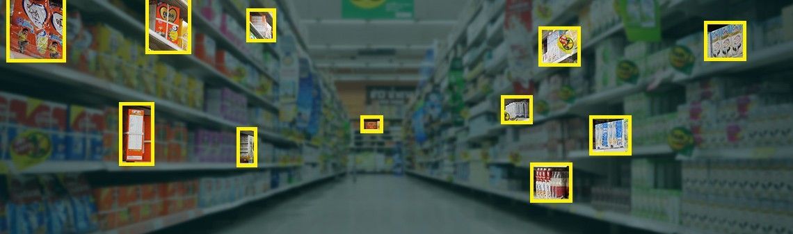
Product recognition is a challenging area that offers great financial promise. Automatically detected product attributes in photos should be easy to monetize, e.g., as a basis for cross-selling and upselling.

However, product recognition is a tough task because the same product can be photographed from different angles, in different lighting, with varying levels of occlusion, etc. Also, different fine-grained product labels, such as ones in royal blue or turquoise, may prove difficult to distinguish visually. Fortunately, properly tuned convolutional neural networks can effectively resolve these problems.
In this post, we discuss our solution for the iMaterialist challenge announced by CVPR and Google and hosted on Kaggle in order to show our approach to product recognition.

The problem

Data and goal

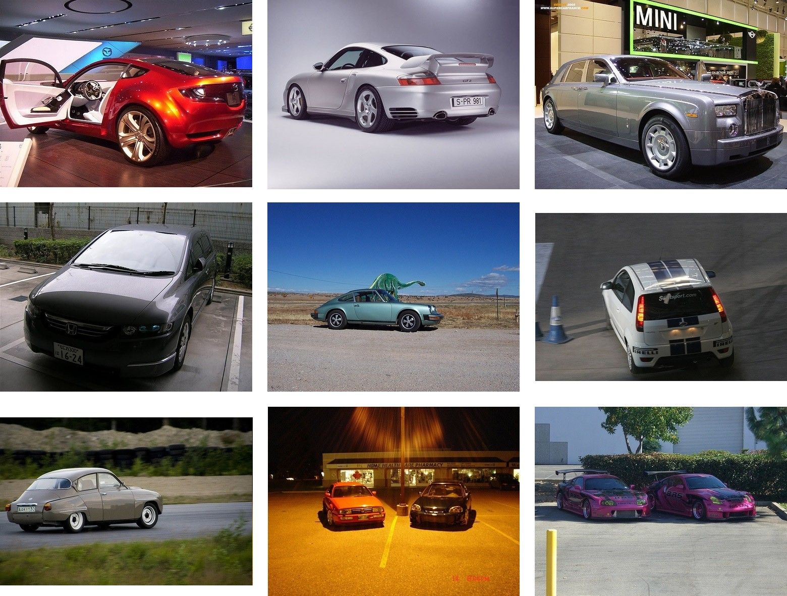
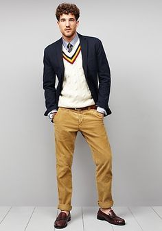
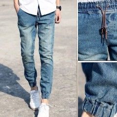
The iMaterialist organizer provided us with hyperlinks to more than 50,000 pictures of shoes, dresses, pants and outerwear. Some tasks were attached to every picture and some labels were matched to every task. Here are some examples:

product recogntion: exemplary picture of dress
task labels
dress: occasion wedding party, cocktail party, cocktail, party, formal, prom
dress: length knee
dress: color dark red, red
product recogntion: exemplary picture of outerwear
task labels
outerwear: age adult
outerwear: type blazers
outerwear: gender men
pants: color brown
product recogntion: exemplary picture of pants
task labels
pants: material jeans, denim, denim jeans
pants: color blue, blue jeans, denim blue, light blue, light, denim
pants: type jeans
pants: age adult
pants: decoration men jeans
pants: gender men
product recogntion: exemplary picture of shoes
task labels
shoe: color dark brown
shoe: up height kneehigh
pants: color black

Our goal was to match a proper label to every task for every picture from the test set. From the machine learning perspective this was a multi-label classification problem.

There were 45 tasks in total (a dozen per cloth type) and we had to predict a label for all of them for every picture. However, tasks not attached to the particular test image were skipped during the evaluation. Actually, usually only a few tasks were relevant to a picture.

Problems with data

There were two main problems with data:

  • We weren’t given the pictures themselves, but only the hyperlinks. Around 10% of them were expired, so our dataset was significantly smaller than the organizer had intended. Moreover, the hyperlinks were a potential source of a data leak. One could use text-classification techniques to take advantage of leaked features hidden in hyperlinks, though we opted not to do that.
  • Some labels with the same meaning were treated by the organizer as different, for example “gray” and “grey”, “camo” and “camouflage”. This introduced noise in the training data and distorted the training itself. Also, we had no choice but to guess if a particular picture from the test set was labeled by the organizer as either “camo” or “camouflage”.

Evaluation

The evaluation score function was the average error over all test pictures and relevant tasks. A score value of 0 meant that all the relevant tasks for all the test pictures were properly labeled, while a score of 1 implied that no relevant task for any picture was labeled correctly. A random sample submission provided by the organizer yielded a score greater than 0.99. Hence we knew that a good result couldn’t be achieved by accident and we would need a model that could actually learn how to solve the problem.

Our solution

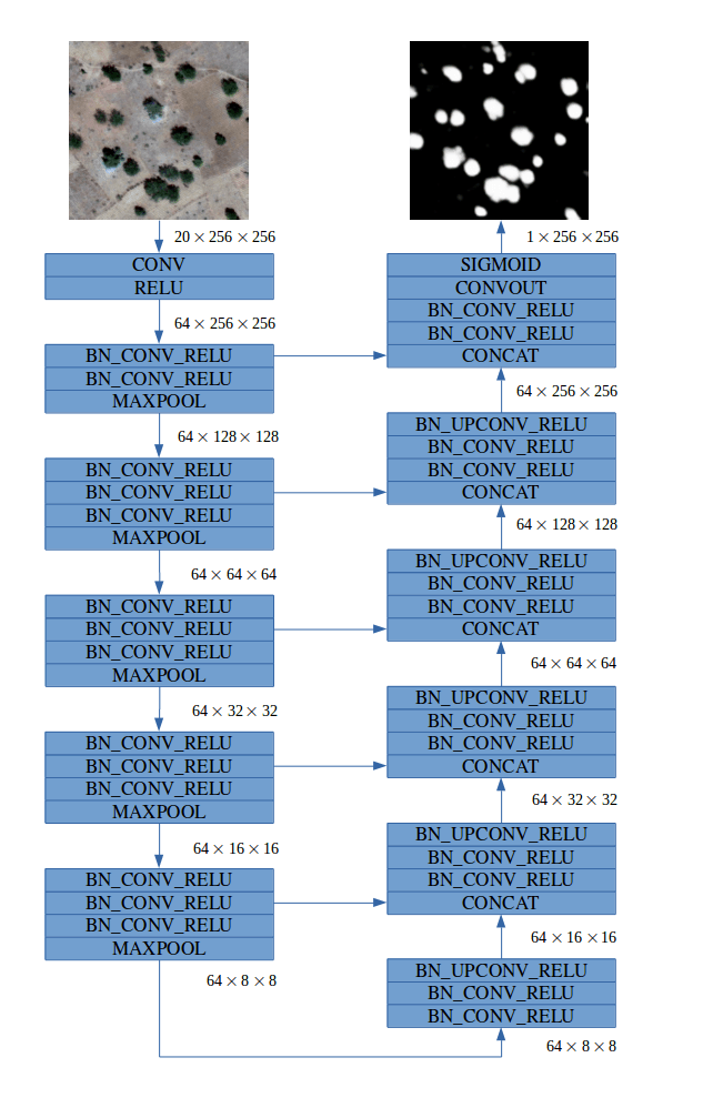
A bunch of convolutional neural networks

Our solution consisted of about 20 convolutional neural networks. We used the following architectures in several variants:

  • DenseNet,
  • ResNet,
  • Inception,
  • VGG.

All of them were initialized with weights pretrained on the ImageNet dataset. Our models also differed in terms of the data preprocessing (cropping, normalizing, resizing, switching of color channels) and augmentation applied (random flips, rotations, color perturbations from Krizhevsky’s AlexNet paper). All the neural networks were implemented using the PyTorch framework.

Choosing the training loss function

Which loss function to choose for the training stage was one of the major problems we faced. 576 unique pairs of task/label occurred in the training data so the outputs of our networks were 576-dimensional. On the other hand, typically only a few labels were matched to  a picture’s tasks. Therefore the ground truth vector was very sparse – only a few of its 576 coordinates were nonzero – so we struggled to choose the right training loss function.
Assume that \((z_1,…,z_{576})in mathbb{R}^{576}\) is a model output and
[y_i=left{begin{array}{ll}1, & text{if task/label pair }itext{ matches the picture,}, & text{elsewhere,}end{array}right.quadtext{for } i=1,2,ldots,576.]

  • As this was a multi-label classification problem,  choosing the popular crossentropy loss function:
    \([sum_{i=1}^{576}-y_ilog p_i,quad text{where } p_i=frac{exp(z_i)}{sum_{j=1}^{576}exp(z_j)},]\)
    wouldn’t be a good idea. This loss function tries to distinguish only one class from others.
  • Also, for the ‘element-wise binary crossentropy’ loss function:
    \([sum_{i=1}^{576}-y_ilog q_i-(1-y_i)log(1-q_i),quad text{where } q_i=frac{1}{1+exp(-z_i)},]\)
    the sparsity caused the models to end up constantly predicting no labels for any picture.
  • In our solution, we used the ‘weighted element-wise crossentropy’ given by:
    \([sum_{i=1}^{576}-bigg(frac{576}{sum_{j=1}^{576}y_j}bigg)cdot y_ilog q_i-(1-y_i)log(1-q_i),quad text{where } q_i=frac{1}{1+exp(-z_i)}.]\)
    This loss function focused the optimization on positive cases.

Ensembling

Predictions from particular networks were averaged, all with equal weights. Unfortunately, we didn’t have enough time to perform any more sophisticated ensembling techniques, like xgboost ensembling.

Other techniques tested

We also tested other approaches, though they proved less successful:

  • Training the triplet network and then training xgboost models on features extracted via embedding (different models for different tasks).
  • Mapping semantically equivalent labels like “gray” and “grey” to a common new label and remapping those to the original ones during postprocessing.
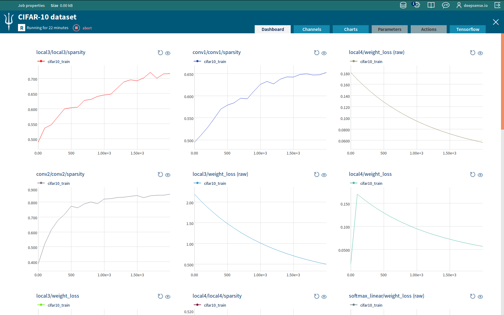
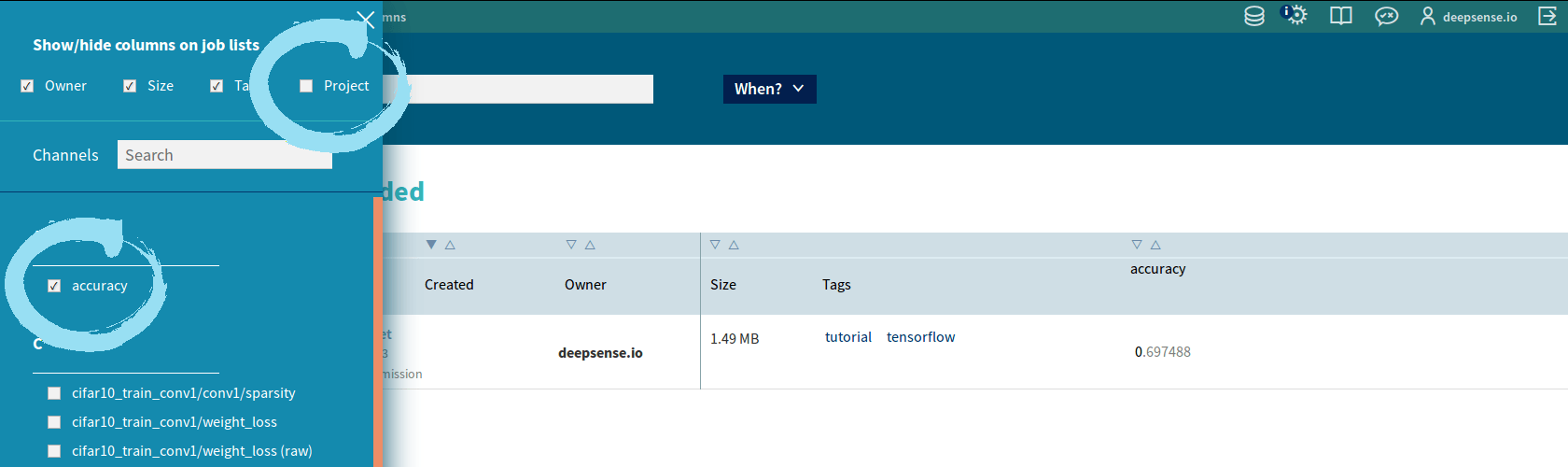
Neptune

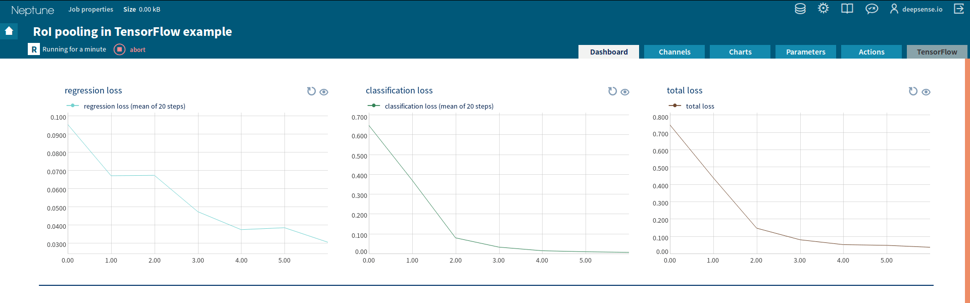
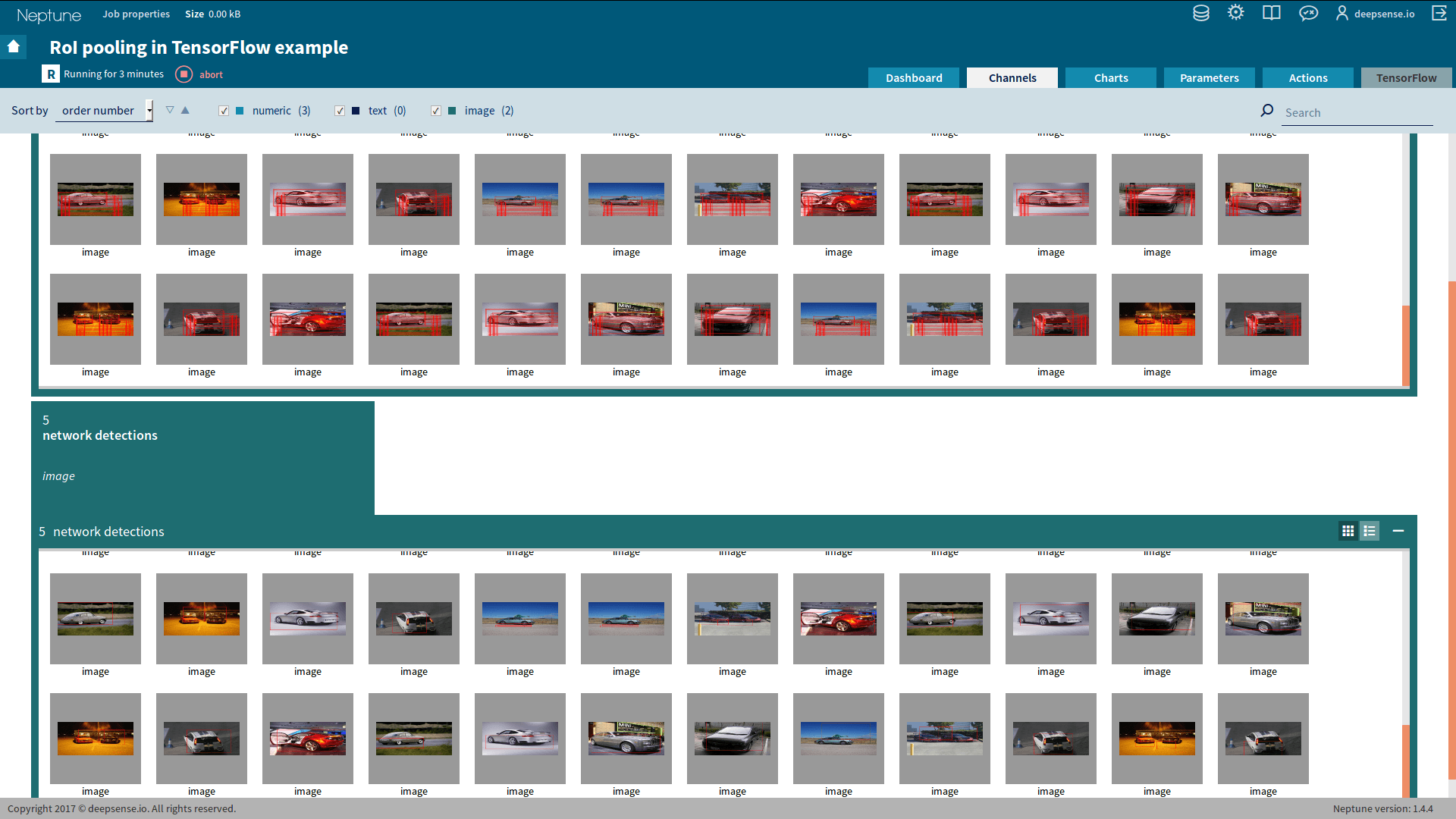
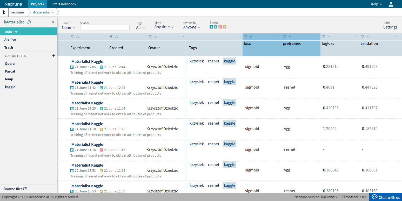
We managed all of our experiments using Neptune, deepsense.ai’s Machine Learning Lab. Thanks to that, we were easily able to track the tuning of our models, compare them and recreate them.
product recogntion: Neptune dashboard

Results

We achieved a score of 0.395, which means that we correctly predicted more than 60% of all the labels matched to relevant tasks.
product recogntion: kaggle leaderboard
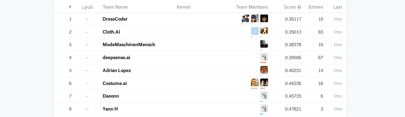
We are pleased with this result, though we could have improved on it significantly if the competition had lasted longer than only one month.

Summary

Challenges like iMaterialist are a good opportunity to create product recognition models. The most important tools and tricks we used in this project were:

  • Playing with training loss functions. Choosing the proper training loss function was a real breakthrough as it boosted accuracy by over 20%.
  • A custom training-validation split. The organizer provided us with a ready-made training-validation split. However, we believed we could use more data for training so we prepared our own split with more training data while maintaining sufficient validation data.
  • Using the PyTorch framework instead of the more popular TensorFlow. TensorFlow doesn’t provide the official pretrained models repository, whereas PyTorch does. Hence working in PyTorch was more time-efficient. Moreover, we determined empirically that, much to our surprise, the same architectures yielded better results when implemented in PyTorch than in TensorFlow.

We hope you have enjoyed this post and if you have any questions, please don’t hesitate to ask!

https://deepsense.ai/wp-content/uploads/2019/02/how-to-create-a-product-recognition-solution.jpg 337 1140 Krzysztof Dziedzic https://deepsense.ai/wp-content/uploads/2019/04/DS_logo_color.svg Krzysztof Dziedzic2017-08-22 13:57:172021-01-05 16:49:37How to create a product recognition solution
Running distributed TensorFlow on Slurm clusters

Running distributed TensorFlow on Slurm clusters

June 26, 2017/in Data science, Deep learning, Machine learning /by Tomasz Grel

In this post, we provide an example of how to run a TensorFlow experiment on a Slurm cluster. Since TensorFlow doesn’t yet officially support this task, we developed a simple Python module for automating the configuration. It parses the environment variables set by Slurm and creates a TensorFlow cluster configuration based on them. We’re sharing this code along with a simple image recognition example on CIFAR-10. You can find it in our github repo.

But first, why do we even need distributed machine learning?

Distributed TensorFlow

When machine learning models are developed, training time is an important factor. Some experiments can take weeks or even months on a single machine. Shortening this time enables us to try out more approaches, test many similar models and use the best one. That’s why it’s useful to use multiple machines for faster training.
One of of TensorFlow’s strongest points is that it’s designed to support distributed computation. To use multiple nodes, you just have to create and start a tf.train.Server and use a tf.train.MonitoredTrainingSession.

Between Graph Replication

In our example we’re going be using a concept called ‘Between Graph Replication’. If you’ve ever run MPI jobs or used the ‘fork’ system call, you’ll be familiar with it.
In Distributed TensorFlow, Between Graph Replication means that when several processes are being run on different machines, each process (worker) runs the same code and constructs the same TensorFlow computational graph. However, each worker uses a discriminator (the worker’s I.D., for example) to execute instructions differently from the rest (e.g. process different batches of the training data).
This information is also used to make processes on some machines work as ‘Parameter Servers’. These jobs don’t actually run any computations – they’re only responsible for storing the weights of the model and sending them over the network to other processes.

Connections between tasks in a distributed TensorFlow job with 3 workers and 2 parameter servers. Note that the workers.

Connections between tasks in a distributed TensorFlow job with 3 workers and 2 parameter servers.

Apart from the worker I.D. and the job type (normal worker or parameter server), TensorFlow also needs to know the network addresses of other workers performing the computations. All this information should be passed as configuration for the tf.train.Server. However, keeping track of it all in addition to starting multiple processes on multiple machines with different parameters can be really tedious. That’s why we have cluster managers, such as Slurm.

Slurm

Slurm is a workload manager for Linux used by many of the world’s fastest supercomputers. It provides the means for running computational jobs on multiple nodes, queuing the jobs until sufficient resources are available and monitoring jobs that have been submitted. For more information about Slurm, you can read the official documentation here.
When running a Slurm job you can discover other nodes taking part by examining environment variables:

  • SLURMD_NODENAME – name of the current node
  • SLURM_JOB_NODELIST – number of nodes the job is using
  • SLURM_JOB_NUM_NODES – list of all nodes allocated to the job

Our python module parses these variables to make using distributed TensorFlow easier. With the tf_config_from_slurm function you can automate this process. Let’s see how it can be used to train a simple CIFAR-10 model on a CPU Slurm cluster.

Distributed TensorFlow on Slurm

In this section we’re going to show you how to run TensorFlow experiments on Slurm. A complete example of training a convolutional neural network on the CIFAR-10 dataset can be found in our github repo, so you might want to take a look at it. Here we’ll just examine the most interesting parts.
Most of the code responsible for training the model comes from this TensorFlow tutorial. The modifications allow the code to be run in a distributed setting on the CIFAR-10 dataset. Let’s examine the changes one by one.

Starting the Server

import tensorflow as tf
from tensorflow_on_slurm import tf_config_from_slurm
cluster, my_job_name, my_task_index = tf_config_from_slurm(ps_number=1)
cluster_spec = tf.train.ClusterSpec(cluster)
server = tf.train.Server(server_or_cluster_def=cluster_spec,
                         job_name=my_job_name, task_index=my_task_index)
if my_job_name == 'ps':
    server.join()
    sys.exit(0)

Here we import our Slurm helper module and use it to create and start the tf.train.Server. The tf_config_from_slurm function returns the cluster spec necessary to create the server along with the task name and task index of the current job. The ‘ps_number’ parameter specifies how many parameter servers to set up (we use 1). All other nodes will be working as normal workers and everything gets passed to the tf.train.Server constructor.
Afterwards we immediately check whether the current job is a parameter server. Since all the work in a parameter server (ps) job is handled by the tf.train.Server (which is running in a separate thread), we can just call server.join() and not execute the rest of the script.

Placing the Variables on a parameter server

def weight_variable(shape):
    with tf.device("/job:ps/task:0"):
        initial = tf.truncated_normal(shape, stddev=0.1)
        return tf.Variable(initial)
def bias_variable(shape):
    with tf.device("/job:ps/task:0"):
        initial = tf.constant(0.1, shape=shape)
        return tf.Variable(initial)

These two functions are used when defining the model parameters. Note the “with tf.device(“/job:ps/task:0”)” statements telling TensorFlow that the variables should be placed on the parameter server, thus enabling them to be shared between the workers. The “0” index denotes the I.D. of the parameter server used to store the variable. Here we’re only using one server, so all the variables are placed on task “0”.

Optimizer

loss = tf.reduce_mean(cross_entropy)
opt = tf.train.AdamOptimizer(1e-3)
opt = tf.train.SyncReplicasOptimizer(opt, replicas_to_aggregate=len(cluster['worker']),
                                     total_num_replicas=len(cluster['worker']))
is_chief = my_task_index == 0
sync_replicas_hook = opt.make_session_run_hook(is_chief)
train_step = opt.minimize(loss, global_step)

Instead of using the usual AdamOptimizer, we’re wrapping it with the SyncReplicasOptimizer. This enables us to prevent the application of stale gradients. In distributed training, the network communication may introduce communication delays which make it harder to train the model.

Creating the session

sync_replicas_hook = opt.make_session_run_hook(is_chief)
sess = tf.train.MonitoredTrainingSession(master=server.target,
                                         is_chief=is_chief,
                                         hooks=[sync_replicas_hook])
batch_size = 64
max_epoch = 10000

In distributed settings we’re using the tf.train.MonitoredTrainingSession instead of the usual tf.Session. This ensures the variables are properly initialized. It also allows you to restore a previously saved model and control how the summaries and checkpoints are written to disk.

Training

During the training, we split the batches between workers so everyone has their own unique batch subset to train on:

for i in range(max_epoch):
    batch = mnist.train.next_batch(batch_size)
    if i % len(cluster['worker']) != my_task_index:
        continue
    _, train_accuracy, xentropy = sess.run([train_step, accuracy, cross_entropy],
                                           feed_dict={x: batch[0], y_: batch[1],
                                           keep_prob: 0.5})


Summary

We hope this example was helpful in your experiments with TensorFlow on Slurm clusters. If you’d like to reproduce it or use our Slurm helper module in your experiments, don’t hesitate to clone our github repo.

https://deepsense.ai/wp-content/uploads/2019/02/tensorflow-on-slurm-clusters.png 337 1140 Tomasz Grel https://deepsense.ai/wp-content/uploads/2019/04/DS_logo_color.svg Tomasz Grel2017-06-26 09:09:382021-02-23 11:19:35Running distributed TensorFlow on Slurm clusters
Machine learning application in automated reasoning

Machine learning application in automated reasoning

May 16, 2017/in Data science, Deep learning, Machine learning /by Przemyslaw Chojecki

It all started with mathematics – rigorous thinking, science, technology. Today’s world is maths‑driven. Despite recent advances in deep learning, the way mathematics is done today is still much the same as it was 100 years ago. Isn’t it time for a change?

Introduction

Mathematics is at the core of science and technology. However the growing amount of mathematical research makes it impossible for non‑experts to fully use the developments made in pure mathematics. Research has become more complicated and more interdependent.
Moreover it is often impossible to verify correctness for non‑experts – knowledge is accepted as knowledge by a small group of experts (e.g. the problem with accepting Mochizuki’s proof of abc‑conjecture – it is not understandable for other experts).

Fig. 1: The graph on the left shows the growing number of submissions to arXiv – an Internet repository for scientific research. In 2012, mathematics accounted for approx. 20,000 submissions annually.

Automated reasoning

To address the issue mentioned above, researchers try to automate or semi‑automate:

  • Producing mathematics
  • Verifying existing mathematics

This domain of science is called automatic theorem proving and is a part of automated reasoning. The current approach to automation is:

  • Take a mathematical work (e.g. Feit‑Thompson theorem or proof of Kepler’s conjecture)
  • Rewrite it in Coq, Mizar or another Interactive Theorem Prover (language/program which understands logic behind mathematics and is able to check its correctness)
  • Verify

The downside to this approach is that it is a purely manual work and quite a tedious process! One has to fill in the gaps as the human way of writing mathematics is different than what Coq/Mizar accepts. Moreover mathematical work is based on previous works. One needs to lay down foundations each time at least to some extent (but have a look at e.g. Mizar Math Library).
Once in Coq/Mizar, there is a growing number of methods to prove new theorems:

  • Hammers and tactics (methods for automatic reasoning over large libraries)
  • Machine learning and deep learning

Here we concentrate on the last method of automated reasoning. Firstly, in order to use the power of machine learning and deep learning, one needs more data. Moreover to keep up with current mathematical research we need to translate LaTeX into Coq/Mizar much faster.

Building a dictionary

We need to automate translation of human‑written mathematical works in LaTeX to Coq/Mizar. We view it as an NLP problem of creating a dictionary between two languages. How can we build such a dictionary? We could build upon existing syntactic parsers (e.g. TensorFlow’s SyntaxNet) and enhance them with Types and variables, which we explain in an example:
Consider the sentence “Let $G$ be a group” . Then “G” is a variable of Type “group”.
Once we have such a dictionary with at least some basic accuracy we can use it to translate LaTeX into Coq/Mizar sentence by sentence. Nevertheless we still need a good source of mathematics! Here is what we propose in the DeepAlgebra program:
Algebraic geometry is one of the pillars of modern mathematical research, which is rapidly developing and has a solid foundation (Grothendieck’s EGA/SGA, The Stacks Project). It is “abstract” hence easier to verify for computers than analytical parts of mathematics.
The Stacks Project is an open multi‑collaboration on foundations of algebraic geometry starting from scratch (category theory and algebra) up to the current research. It has a well‑organized structure (an easy‑to‑manage dependency graph) and is verified thoroughly for correctness.
The Stacks Project now consists of:

  • 547,156 lines of code
  • 16,738 tags (57 inactive tags)
  • 2,691 sections
  • 99 chapters
  • 5,712 pages
  • 162 slogans

Moreover it has an API to query!

  • Statements (also in LaTeX)
  • Data for graphs

Below we present a few screenshots.

Fig. 2: One of the lemmas in the Stacks Project. Each lemma has a unique tag (here 01WC), which never changes, even though the number of the lemma may change. Each lemma has a proof and we can access its dependency graphs:


Figs. 3 and 4: Two dependency graphs for Lemma 01WC, which show the structure of the proof together with all the lemmas, propositions and definitions which were used along the way.

Conclusion

Summing up, we propose to treat the Stacks Project as a source of data for NLP research and eventual translation into one of the Interactive Theorem Provers. The first step in the DeepAlgebra program is to build a dictionary (syntactic parser with Types/variables) and then test it on the Stacks Project. This way we would build an “ontology” of algebraic geometry. If that works out, we can verify, modify and test it on arXiv (Algebraic Geometry submissions). We will report on our progress in automated reasoning in future texts.

This text was based on https://arxiv.org/abs/1610.01044
The author presented this material at AITP conference – http://aitp-conference.org/2017/

https://deepsense.ai/wp-content/uploads/2019/02/Machine-learning-application-in-automated-reasoning.jpg 337 1140 Przemyslaw Chojecki https://deepsense.ai/wp-content/uploads/2019/04/DS_logo_color.svg Przemyslaw Chojecki2017-05-16 10:50:532021-01-05 16:49:47Machine learning application in automated reasoning

Region of interest pooling in TensorFlow – example

April 25, 2017/in Data science, Deep learning, Machine learning, Neptune /by Krzysztof Dziedzic, Patryk Miziuła and Błażej Osiński

In the previous post we explained what region of interest pooling (RoI pooling for short) is. In this one, we present an example of applying RoI pooling in TensorFlow. We base it on our custom RoI pooling TensorFlow operation. We also use Neptune as a support in our experiment performance tracking.

Example overview

Our goal is to detect cars in the images. We’d like to construct a network that is able to automatically draw a box around every car.
In our example we deal with car images from the Pascal VOC 2007 dataset. For simplicity we choose only cars not marked as truncated.

Exemplary images from Pascal VOC 2007 dataset
Related:  Region of interest pooling explained

Neptune

We manage our experiment using Neptune. It’s a pretty handy tool:

  • We track the tuning in real time. Especially, we preview the currently estimated bounding boxes.
  • We can change model hyperparameters on the fly.
  • We can easily integrate Neptune with TensorFlow and get all the charts, graphs and summary objects from the TensorFlow graph.
  • We store the executed experiments in an aesthetic list.

Network architecture

In our example we use the Fast R-CNN architecture.
The network has two inputs:

  1. Batch of images
  2. Batch of potential bounding boxes – RoI proposals
    In the Fast R-CNN model RoI proposals are generated via an external algorithm, for example selective search. In our example, we take ground truth bounding boxes from the Pascal annotations and generate more negative bounding boxes ourselves.

The network has two outputs:

  1. Batch of RoI proposals not classified as background (with corrected coordinates)
  2. Probabilities that RoI proposals consist of objects of the consecutive categories

The network consists of three main parts:

  1. Deep convolutional neural network
    • Input: images
    • Output: feature map

    We use the popular VGG16 network pretrained on the ImageNet dataset.

  2. RoI pooling layer
    • Input: feature map, RoI proposals resized to a feature map
    • Output: max-pooled RoI proposals
  3. Fully connected layer with RoI features
    • Input: max-pooled RoI proposals
    • Output: corrected RoI proposals, probabilities
RoI pooling in TensorFlow scheme
Fast R-CNN architecture

We note that our detection task can be also solved with the Faster R-CNN architecture, which works significantly faster :). However, the implementation of Faster R-CNN requires much more code to write, so we chose the simpler Fast R-CNN.

Loss function

We tune the network to minimize the loss given by
\(loss = frac 1nsum_{i=1}^n frac 1{k_i} sum_{j=1}^{k_i} loss_{ij}\)
where:

  • \(n\) is a number of images in a batch,
  • \(k_i\) is a number of RoI proposals for the image \(i\),
  • \(loss_{ij}\) is a loss for the RoI proposal \(j\) for the image \(i\).

For a single RoI proposal, \(loss_{ij}\) is the sum of the classification and regression loss, where:

  • classification loss is the common cross entropy,
  • regression loss is a smooth L1 distance between the rescaled coordinates of a RoI proposal and the ground-truth box. The regression loss is computed if the ground-truth box is not categorized as background, otherwise it’s defined as 0.
Related:  Playing Atari with deep reinforcement learning - deepsense.ai’s approach

Implementation details

Prerequisites

To run the code we provide, you need the following software:

  • CUDA 8,
  • TensorFlow 1.0 with GPU support,
  • our custom RoI pooling TensorFlow operation,
  • OpenCV,
  • Neptune (version 1.5): apply for our Early Adopters Program or try it immediately with Neptune Go.

Repository

You can download our code from our GitHub repository. It consists of two folders with the following content:

File Purpose
code
main.py The script to execute.
fast_rcnn.py Builds the TensorFlow graph.
trainer.py Preprocesses data and trains the network.
neptune_handler.py Contains Neptune utilities.
config.yaml Neptune configuration file.
get_data.py Downloads images from Pascal VOC 2007 dataset
data
vgg16-20160129.tfmodel.torrent References to weights of the pretrained network.

Description

When we run main.py , the script trainer.py  first restores the VGG16 network with the pretrained weights. Then it adds the RoI pooling layer and the fully connected layer. Finally, it begins tuning the entire network with use of provided images and RoI proposals. It also sends information to Neptune, so we can track the tuning progress in real time.
After cloning the repository, please download the file vgg16-20160129.tfmodel  referred to by the torrent file vgg16-20160129.tfmodel.torrent  and save it in the data  directory. Also, please run the script get_data.py to download needed images:

python get_data.py

Let’s test our RoI pooling in TensorFlow!

We run the script main.py  from the code folder by typing:

neptune run --
            --im_folder $PWD/../data/images
            --roidb $PWD/../data/roidb
            --pretrained_path $PWD/../data/vgg16-20160129.tfmodel

If we want to also use a non-default learning rate value or the number of epochs, we can add:

--learning_rate 1e-03 --num_epochs 200

to the command at the end.
After a while, we can start observing the tuning progress in Neptune:

RoI pooling in TensorFlow - tuning
Tracking the network tuning in Neptune

Moreover, we can display the RoIs fitted to the cars by our network. We could just load all the processed images, but this procedure would take much of resources. That’s why we decided to activate this feature by a simple Neptune action.
To do that, we can go to the Actions tab and click ‘RUN’ to start sending the images.

RoI pooling in TensorFlow - turning on the image sending in Neptune
Turning on the image sending

After that, we can go to the Channels tab and expand the channels ‘region proposals for RoI pooling’ and ‘network detections’ by clicking ‘+’ signs.

Roi pooling in TensorFlow - expanding image channels in Neptune
Expanding image channels

Now we can see the RoIs in real time!

RoI pooling in TensorFlow - RoI preview
RoI proposals preview in Neptune

We can click on the pictures to zoom them. If we want Neptune to stop sending new images, we go to the Actions tab and click ‘RUN’ again.
An exemplary NeptuneGo execution of our script can be found here.

Related:  Logo detection and brand visibility analytics - example

Summary

We hope you enjoy our example of RoI pooling in TensorFlow and experiment managing features offered by Neptune. If you want to comment our work, don’t be hesitate to leave us feedback!

References

  • R. Girshick, Fast R-CNN, IEEE International Conference on Computer Vision (ICCV), 2015.
  • S. Ren, K. He, R. Girshick & J. Sun, Faster R-CNN: towards real-time object detection with Region Proposal Networks, Neural Information Processing Systems (NIPS), 2015.
  • deepsense.ai, Region of interest pooling explained, 2017.
https://deepsense.ai/wp-content/uploads/2019/02/roi-pooling-in-tensorflow-example.jpg 337 1140 Krzysztof Dziedzic https://deepsense.ai/wp-content/uploads/2019/04/DS_logo_color.svg Krzysztof Dziedzic2017-04-25 11:46:062021-01-05 16:49:52Region of interest pooling in TensorFlow – example
Neptune 1.5 - Python 3 support, simplified CLI, compact view

Neptune 1.5 – Python 3 support, simplified CLI, compact view

April 21, 2017/in Data science, Deep learning, Machine learning, Neptune /by Rafał Hryciuk

At the end of April 2017, deepsense.ai released a new version of Neptune, the DevOps platform for data scientists. Neptune 1.5 introduces a range of new features and improvements, including support for Python 3, simplification of Neptune CLI, offline execution, compact view, improved channels and charts, and a number of improvements in the user experience.

Python 3.5 Support

One of the most upvoted tickets on our feedback channel has been requests to add support for Python 3. Well, we put your request on our roadmap and now, using version 1.5, you can run Neptune experiments using both Python 2.7 and 3.5.
We encourage you to stay active in our feedback forum and vote for features you need in your data science work. This is how you will influence where Neptune goes and how it develops – and ultimately make it more convenient for you.

Simplification of Neptune CLI

Until now, Neptune CLI’s commands were long and complex. With version 1.5, however, convenience has taken center stage as we’ve introduced a host of improvements and simplifications. Click over and have a look at the simplified CLI commands and configuration file in our documentation.
To see how this change could work for you, compare the commands for running our “Flower Species Prediction” example.
In version 1.4:

neptune run flower-species-prediction/main.py --config flower-species-prediction/config.yaml --storage-url /tmp/neptune-iris --paths-to-dump flower-species-prediction

In version 1.5:

neptune run

Offline Execution

Our users often run parts of their experiments using Jupyter Notebook, but the Neptune client library requires communication with our server. Thanks to offline execution, users can disable communication with the server and run their experiments without CLI. Read more about this convenient development here.

Compact View

To make comparing your experiments easier we have introduced a compact view of the experiments table. You can now display more experiment results on your screen, and draw conclusions even faster and more confidently.

Improved Channels and Charts

Neptune 1.5 comes with the new API for channels and charts. Thanks to the new API you will be able to send and display even more data points. Your charts will load faster and more seamlessly. We encourage you to give the improved channels and charts a go.

The Neptune Pipeline

We are already working on the next version of Neptune, which is slated for a May release and will focus on better displaying the experiments list.
We hope you will enjoy working with our DevOps platform for data scientists. Neptune 1.5 will help you manage and monitor your machine learning experiments even more conveniently.
Would you like to test drive Neptune? Visit NeptuneGo!, have a look around and run your first experiments.

NeptuneGo!

https://deepsense.ai/wp-content/uploads/2019/02/neptune-1-5-python-3-support-simplified-cli-compact-view.jpg 337 1140 Rafał Hryciuk https://deepsense.ai/wp-content/uploads/2019/04/DS_logo_color.svg Rafał Hryciuk2017-04-21 13:50:212021-01-05 16:49:56Neptune 1.5 – Python 3 support, simplified CLI, compact view
Deep learning for satellite imagery via image segmentation

Deep learning for satellite imagery via image segmentation

April 12, 2017/in Data science, Deep learning, Machine learning /by Arkadiusz Nowaczynski

In the recent Kaggle competition Dstl Satellite Imagery Feature Detection our deepsense.ai team won 4th place among 419 teams. We applied a modified U-Net – an artificial neural network for image segmentation. In this blog post we wish to present our deep learning solution and share the lessons that we have learnt in the process with you.

Competition

The challenge was organized by the Defence Science and Technology Laboratory (Dstl), an Executive Agency of the United Kingdom’s Ministry of Defence on Kaggle platform. As a training set, they provided 25 high-resolution satellite images representing 1 km2 areas. The task was to locate 10 different types of objects:

  1. Buildings
  2. Miscellaneous manmade structures
  3. Roads
  4. Tracks
  5. Trees
  6. Crops
  7. Waterway
  8. Standing water
  9. Large vehicles
  10. Small vehicles

Satellite imagery sample with labels.

Sample image from the training set with labels.

These objects were not completely disjoint – you can find examples with vehicles on roads or trees within crops. The distribution of classes was uneven: from very common, such as crops (28% of the total area) and trees (10%), to much smaller such as roads (0.8%) or vehicles (0.02%). Moreover, most images only had a subset of classes.

Correctness of prediction was calculated using Intersection over Union (IoU, known also as Jaccard Index) between predictions and the ground truth. A score of 0 meant complete mismatch, whereas 1 – complete overlap. The score result was calculated for each class separately and then averaged. For our solution the average IoU was 0.46, whereas for the winning solution it was 0.49.

Related:  Five hottest big data trends 2018 for the techies

Preprocessing

For each image we were given three versions: grayscale, 3-band and 16-band. Details are presented in the table below:

Type Wavebands Pixel resolution #channels Size
grayscale Panchromatic 0.31 m 1 3348 x 3392
3-band RGB 0.31 m 3 3348 x 3392
16-band Multispectral 1.24 m 8 837 x 848
Short-wave infrared 7.5 m 8 134 x 136

We resized and aligned 16-band channels to match those from 3-band channels. Alignment was necessary to remove shifts between channels. Finally all channels were concatenated into single 20-channels input image.

Model

Our fully convolutional model was inspired by the family of U-Net architectures, where low-level feature maps are combined with higher-level ones, which enables precise localization. This type of network architecture was especially designed to effectively solve image segmentation problems. U-Net was the default choice for us and other competitors. If you would like more insights into architecture we suggest that you read the original paper. Our final architecture is depicted below:
Convolutional neural network for image segmentation in satellite imagery.For more details about specific modules click here.
Typical convolutional neural network (CNN) architecture involves increasing the number of feature maps (channels) with each max pooling operation. In our network we decided to keep a constant number of 64 feature maps throughout the network. This choice was motivated by two observations. Firstly, we can allow the network to lose some information after the downsampling layer because the model has access to low level features in the upsampling path. Secondly, in satellite images there is no concept of depth or high-level 3D objects to understand, so a large number of feature maps in higher layers may not be critical for good performance.
We developed separate models for each class, because it was easier to fine tune them individually for better performance and to overcome imbalanced data problems.

Training procedure

Models assign probability of belonging to a target class for each pixel from the input image. Although Jaccard was the evaluation metric, we used the per-pixel binary cross entropy objective for training.
We normalized images to have a zero mean and unit variance using precomputed statistics from the dataset. Depending on class we left preprocessed images unchanged or resized them together with corresponding label masks to 1024 x 1024 or 2048 x 2048 squares. During training we collected a batch of cropped 256 x 256 patches from different images where half of the images always contained some positive pixels (objects of target classes). We found this to be both the best and the simplest way to handle the imbalanced classes problem. Each image in a batch was augmented by randomly applying horizontal and vertical flips together with random rotation and color jittering.
Each model had approx. 1.7 million parameters. Its training (with batch size 4) from scratch took about two days on a single GTX 1070.

Related:  Image classification sample solution for Kaggle competition

Predictions

We used a sliding window approach at test time with window size fixed to 256 x 256 and stride of 64. This allowed us to eliminate weaker predictions on image patch boundaries where objects may only be partially shown without context around them. To further improve prediction quality we averaged results for flipped and rotated versions of the input image, as well as for models trained on different scales. Overall we obtained well smoothed outputs.

Post-processing

Ground truth labels were provided in WKT format, presenting objects as polygons (defined by their vertices). It was necessary for us to generate submissions where polygons are concise and can be processed quickly by the evaluation system to avoid timeout limits. We found that this can be accomplished with minimal loss on the evaluation metric by using parameterized operations on binarized outputs. In our post-processing stage we used morphology dilation/erosion and simply removed objects/holes smaller than a given threshold.

Our solution

Buildings, Misc., Roads, Tracks, Trees, Crops, Standing Water

For these seven classes we were able to train convolutional networks (separately for each class) with binary cross entropy loss as described above on 20 channels inputs and two different scales (1024 and 2048) with satisfactory results. Outputs of the models were simply averaged and then post-processed with hyperparameters depending on particular classes.

Waterway

The solution for the waterway class was a combination of linear regression and random forest, trained on per pixel data from 20 input channels. Such a simple setup works surprisingly well because of the characteristic spectral response of water.

Large and Small Vehicles

We observed high variation of the results on the local validation and public leaderboard due to the small number of vehicles in the training set. To combat this we trained models separately for large and small vehicles, as well as single model for both of them (label masks were added together) on 20 channels inputs. Additionally, we repeated all experiments using 4 channels inputs (RGB + Panchromatic) to increase diversity of our models in ensemble. Outputs from models trained on both classes were averaged with single class specific models to produce final predictions for each type of vehicles.

Technologies

We implemented models in PyTorch and Keras (with TensorFlow backend), according to our team members’ preferences. Our strategy was to build separate models for each class, so this required careful management of our code. To run models and keep track of our experiments we used Neptune.

Related:  Playing Atari with deep reinforcement learning - deepsense.ai’s approach

Final results

Below we present a small sample of the final results from our models:

Buildings detection in satellite imagery.

Buildings

Roads detection in satellite imagery.

Roads

Tracks detection in satellite imagery.

Tracks

Crops detection in satellite imagery.

Crops

Waterway detection in satellite imagery.

Waterway

Small vehicles detection in satellite imagery.

Small vehicles

Conclusions

Satellite imagery is a domain with a high volume of data which is perfect for deep learning. We have proved that the results gained from current state-of-the-art research can be applied to solve practical problems. Excited by our results, we look forward to more of such challenges in the future.
Team members:
Arkadiusz Nowaczyński
Michał Romaniuk
Adam Jakubowski
Michał Tadeusiak
Konrad Czechowski
Maksymilian Sokołowski
Kamil Kaczmarek
Piotr Migdał

Suggested readings

For those of you interested in additional reading, we recommend the following papers on image segmentation which inspired our work and success:

  1. Fully Convolutional Networks for Semantic Segmentation
  2. U-Net: Convolutional Networks for Biomedical Image Segmentation
  3. The One Hundred Layers Tiramisu: Fully Convolutional DenseNets for Semantic Segmentation
  4. Analyzing The Papers Behind Facebook’s Computer Vision Approach
  5. Image-to-Image Translation with Conditional Adversarial Nets
  6. ReSeg: A Recurrent Neural Network-based Model for Semantic Segmentation
https://deepsense.ai/wp-content/uploads/2019/02/deep-learning-for-satellite-imagery-via-image-segmentation.jpg 337 1140 Arkadiusz Nowaczynski https://deepsense.ai/wp-content/uploads/2019/04/DS_logo_color.svg Arkadiusz Nowaczynski2017-04-12 13:39:182021-01-05 16:50:01Deep learning for satellite imagery via image segmentation
Neptune machine learning platform: grid search, R & Java support

Neptune machine learning platform: grid search, R & Java support

March 6, 2017/in Data science, Deep learning, Machine learning, Neptune /by Rafał Hryciuk

In February we released a new version of Neptune, our machine learning platform for data scientists, supporting them in more efficient experiment management and monitoring. The latest 1.4 release introduces new features, like grid search — a hyperparameter optimization method and support for R and Java programming languages.

Grid Search

The first major feature introduced in Neptune 1.4 is support for grid search, which is one of the most popular hyperparameter optimization method. You can read more about grid search here.
In version 1.4 in your Neptune experiment you can pass a list or a range of values instead of passing a specific value for the numeric parameter. Neptune will create a grid search experiment and run a job for every combination of parameters’ values. Neptune groups and helps you manage results within the grid search experiment. You can define custom metrics for evaluation. Neptune will automatically select the combination of hyperparameters’ values that give the best value of the metric. Read an example.

R Support and Java Support

Neptune exposes REST API, so it is completely language and platform agnostic. deepsense.ai provides high-level client libraries for the most popular programming languages among data scientists (according to the poll taken in the community — see the results). Thanks to client libraries, users don’t have to implement communication via REST API themselves but instead they can invoke high-level functions. Until version 1.4 we only supported client library for Python. In version 1.4 we introduced support for for R and Java (which also covers Scala users). Thanks to new client libraries you can run, monitor and manage your experiments written in R or Java in the Neptune machine learning platform. You can get client libraries for R and Java here.

Future Plans

We have already been working on the next version of Neptune, which will be released at the beginning of April 2017. Next release will contain:

  • Architectural and API changes that will improve user experience.
  • New approach for handling snapshots of the experiments’ code.
  • Neptune Offline Context — the user will be able to run the code that uses Neptune API offline.

I hope you will enjoy working with our machine learning platform, now with grid search support and client libraries for R and Java. If you’d like to give us feedback, feel free to use our forum at https://community.neptune.ml.
Do you want to check out Neptune? Visit NeptuneGo!, look around and run your first experiments.

https://deepsense.ai/wp-content/uploads/2019/02/neptune-machine-learning-platform-grid-search-r-java-support.jpg 337 1140 Rafał Hryciuk https://deepsense.ai/wp-content/uploads/2019/04/DS_logo_color.svg Rafał Hryciuk2017-03-06 12:57:132021-01-05 16:50:12Neptune machine learning platform: grid search, R & Java support
Region of interest pooling explained

Region of interest pooling explained

February 28, 2017/in Data science, Deep learning, Machine learning /by Tomasz Grel

Region of interest pooling (also known as RoI pooling) is an operation widely used in object detection tasks using convolutional neural networks. For example, to detect multiple cars and pedestrians in a single image. Its purpose is to perform max pooling on inputs of nonuniform sizes to obtain fixed-size feature maps (e.g. 7×7).

We’ve just released an open-source implementation of RoI pooling layer for TensorFlow (you can find it here). In this post, we’re going to say a few words about this interesting neural network layer. But first, let’s start with some background.
Two major tasks in computer vision are object classification and object detection. In the first case the system is supposed to correctly label the dominant object in an image. In the second case it should provide correct labels and locations for all objects in an image. Of course there are other interesting areas of computer vision, such as image segmentation, but today we’re going to focus on detection. In this task we’re usually supposed to draw bounding boxes around any object from a previously specified set of categories and assign a class to each of them. For example, let’s say we’re developing an algorithm for self-driving cars and we’d like to use a camera to detect other cars, pedestrians, cyclists, etc. — our dataset might look like this.
In this case we’d have to draw a box around every significant object and assign a class to it. This task is more challenging than classification tasks such as MNIST or CIFAR. On each frame of the video, there might be multiple objects, some of them overlapping, some poorly visible or occluded. Moreover, for such an algorithm, performance can be a key issue. In particular for autonomous driving we have to process tens of frames per second.
So how do we solve this problem?

Related:  Playing Atari with deep reinforcement learning - deepsense.ai’s approach

Typical architecture

The object detection architecture we’re going to be talking about today is broken down in two stages:

  1. Region proposal: Given an input image find all possible places where objects can be located. The output of this stage should be a list of bounding boxes of likely positions of objects. These are often called region proposals or regions of interest. There are quite a few methods for this task, but we’re not going to talk about them in this post.
  2. Final classification: for every region proposal from the previous stage, decide whether it belongs to one of the target classes or to the background. Here we could use a deep convolutional network.


Object detection pipeline wit region of interest pooling

Object detection pipeline with region of interest pooling

Usually in the proposal phase we have to generate a lot of regions of interest. Why? If an object is not detected during the first stage (region proposal), there’s no way to correctly classify it in the second phase. That’s why it’s extremely important for the region proposals to have a high recall. And that’s achieved by generating very large numbers of proposals (e.g., a few thousands per frame). Most of them will be classified as background in the second stage of the detection algorithm.
Some problems with this architecture are:

  • Generating a large number of regions of interest can lead to performance problems. This would make real-time object detection difficult to implement.
  • It’s suboptimal in terms of processing speed. More on this later.
  • You can’t do end-to-end training, i.e., you can’t train all the components of the system in one run (which would yield much better results)

That’s where region of interest pooling comes into play.

Related:  Optimize Spark with DISTRIBUTE BY & CLUSTER BY

Region of interest pooling — description

Region of interest pooling is a neural-net layer used for object detection tasks. It was first proposed by Ross Girshick in April 2015 (the article can be found here) and it achieves a significant speedup of both training and testing. It also maintains a high detection accuracy. The layer takes two inputs:

  1. A fixed-size feature map obtained from a deep convolutional network with several convolutions and max pooling layers.
  2. An N x 5 matrix of representing a list of regions of interest, where N is a number of RoIs. The first column represents the image index and the remaining four are the coordinates of the top left and bottom right corners of the region.


region proposals on a cat image An image from the Pascal VOC dataset annotated with region proposals (the pink rectangles)

What does the RoI pooling actually do? For every region of interest from the input list, it takes a section of the input feature map that corresponds to it and scales it to some pre-defined size (e.g., 7×7). The scaling is done by:

  1. Dividing the region proposal into equal-sized sections (the number of which is the same as the dimension of the output)
  2. Finding the largest value in each section
  3. Copying these max values to the output buffer

The result is that from a list of rectangles with different sizes we can quickly get a list of corresponding feature maps with a fixed size. Note that the dimension of the RoI pooling output doesn’t actually depend on the size of the input feature map nor on the size of the region proposals. It’s determined solely by the number of sections we divide the proposal into. What’s the benefit of RoI pooling? One of them is processing speed. If there are multiple object proposals on the frame (and usually there’ll be a lot of them), we can still use the same input feature map for all of them. Since computing the convolutions at early stages of processing is very expensive, this approach can save us a lot of time.

Related:  Deep learning for satellite imagery via image segmentation

Region of interest pooling — example

Let’s consider a small example to see how it works. We’re going to perform region of interest pooling on a single 8×8 feature map, one region of interest and an output size of 2×2. Our input feature map looks like this:
Region of interest pooling example (input feature map)
Let’s say we also have a region proposal (top left, bottom right coordinates): (0, 3), (7, 8). In the picture it would look like this:
Region of interest pooling example (region proposal)Normally, there’d be multiple feature maps and multiple proposals for each of them, but we’re keeping things simple for the example.
By dividing it into (2×2) sections (because the output size is 2×2) we get:
Region of interest pooling example (pooling sections)
Notice that the size of the region of interest doesn’t have to be perfectly divisible by the number of pooling sections (in this case our RoI is 7×5 and we have 2×2 pooling sections).
The max values in each of the sections are:
Region of interest pooling example (output)
And that’s the output from the Region of Interest pooling layer. Here’s our example presented in form of a nice animation:
Region of interest pooling (animation)
What are the most important things to remember about RoI Pooling?

  • It’s used for object detection tasks
  • It allows us to reuse the feature map from the convolutional network
  • It can significantly speed up both train and test time
  • It allows to train object detection systems in an end-to-end manner

If you need an opensource implementation of RoI pooling in TensorFlow you can find our version here.
In the next post, we’re going to show you some examples on how to use region of interest pooling with Neptune and TensorFlow.

References:

  • Girshick, Ross. “Fast r-cnn.” Proceedings of the IEEE International Conference on Computer Vision. 2015.
  • Girshick, Ross, et al. “Rich feature hierarchies for accurate object detection and semantic segmentation.” Proceedings of the IEEE conference on computer vision and pattern recognition. 2014.
  • Sermanet, Pierre, et al. “Overfeat: Integrated recognition, localization and detection using convolutional networks.” arXiv preprint arXiv:1312.6229. 2013.
https://deepsense.ai/wp-content/uploads/2019/02/region-of-interest-pooling-explained.jpg 337 1140 Tomasz Grel https://deepsense.ai/wp-content/uploads/2019/04/DS_logo_color.svg Tomasz Grel2017-02-28 14:46:472021-04-14 18:06:40Region of interest pooling explained
An internal validation leaderboard in Neptune

An internal validation leaderboard in Neptune

January 19, 2017/in Data science, Deep learning, Machine learning, Neptune /by Patryk Miziuła

Internal validation is a useful tool for comparing results of experiments performed by team members in any business or research task. It can also be a valuable complement of public leaderboards attached to machine learning competitions on platforms like Kaggle.

In this post, we present how to build an internal validation leaderboard using Python scripts and the Neptune environment. As an example of a use case, we will take the well known classification dataset CIFAR-10. We study it using a deep convolutional neural network provided in the TensorFlow tutorial.

Why internal leaderboard?

Whenever we solve the same problem in many ways, we want to know which way is the best. Therefore we validate, compare and order the solutions. In this way, we naturally create the ranking of our solutions – the leaderboard.
We usually care about the privacy of our work. We want to keep the techniques used and the results of our experiments confidential. Hence, our validation should remain undisclosed as well – it should be internal.
If we keep improving the models and produce new solutions at a fast pace, at some point we are no longer able to manage the internal validation leaderboard manually. Then we need a tool which will do that for us automatically and will present the results to us in a readable form.

Business and research projects

In any business or research project you are probably interested in the productivity of team members. You would like to know who and when submits his or her solution to the problem, what kind of model they use and how good the solution is.
A good internal leaderboard stores all that information. It also allows you to search for submissions sent by specific user, defined in some time window or using a particular model. Finally, you can sort the submissions with respect to the accuracy metric to find the best one.

Machine learning competitions

The popular machine learning platform, Kaggle, offers a readable public leaderboard for every competition. Each contestant can follow his position in the ranking and try to improve several times a day.
However, an internal validation would be very useful for every competing team. A good internal leaderboard has many advantages over a public one:

  • the results remain exclusive,
  • there is no limit on the number of daily submissions,
  • metrics other than those chosen by the competition organizers can be evaluated as well,
  • the submissions can be tagged, for example to indicate the used model.

Note that in every official competition the ground truth labels for the test data are not provided. Hence, to produce the internal validation we are forced to split the available public training data. One part is used to tune the model, the other is needed to evaluate it internally. This division can be an origin of unexpected problems (e.g., data leaks) so perform it carefully!

Why Neptune?

Neptune was designed to manage multiple experiments. Among many features, it supports storing parameters, logs and metric values from various experiment executions. The results are accessible through an aesthetic Web UI.
In Neptune you can:

  • gather experiments from various projects in groups,
  • add tags to experiments and filter by them,
  • sort experiments by users, date of creation, or – most importantly for us – by metric values.

Due to that, Neptune is a handy tool for creating an internal validation leaderboard for your team.

An internal validation leaderboard in Neptune

Tracking a TensorFlow experiment in Neptune

Let’s do it!

Let’s build an exemplary internal validation leaderboard in Neptune.

CIFAR-10 dataset

We use the well-known classification dataset CIFAR-10. Every image in this dataset is a member of one of 10 classes, labeled by numbers from 0 to 9. Using the train data we build a model which allows us to predict the labels of images from test data. CIFAR-10 is designed for educational purposes, therefore the ground truth labels for test data are provided.

Evaluating functions

Let’s fix the notation:

  • \(N\) – number of images we have to classify.
  • \(c_i\) – class to which the \(i\)th image belongs; \(iin{0,ldots,N-1}\), \(c_iin{0,ldots,9}\).
  • \(p_{ij}\) – estimated probability that the \(i\)th image belongs to the class \(j\); \(iin{0,ldots,N-1}\), \(jin{0,ldots,9}\), \(p_{ij}in[0,1]\).

We evaluate our submission with two metrics. The first metric is the classification accuracy given by
\(frac 1Nsum_{i=0}^{N-1}mathbb{1}Big(argmax_j p_{ij}=c_iBig)\)
This is the percentage of labels that are predicted correctly. We would like to maximize it, the optimal value is 1. The second metric is the average cross entropy given by
\(-frac 1Nsum_{i=0}^{N-1}log p_{ic_i}\)
This formula is simpler than the principal entropy since the classes are completely mutually exclusive. We would like to minimize it, preferably to 0.

Implementation details

Prerequisites

To run the code we provide you need the following software:

  • Neptune: apply for our Early Adopters Program or try it immediately with Neptune Go,
  • TensorFlow 1.0.

Repository

The code we use is based on that available in the TensorFlow convolutional neural networks tutorial. You can download our code from our GitHub repository. It consists of the following files:

File Purpose
main.py The script to execute.
cifar10_submission.py Computes submission for a CIFAR-10 model.
evaluation.py Contains functions required to create the leaderboard in Neptune.
config.yaml Neptune configuration file.

Description

When you run main.py, you first train a neural network using function cifar10_train provided by TensorFlow. We hard-coded the number of training steps. This could be enhanced to dynamic using Neptune action, but for the sake of brevity we skip this topic in the blog post. Due to TensorFlow Integration you can track the tuning of the network in Neptune. Moreover, the parameters of the tuned network are stored in a file manageable by TensorFlow saver objects.
Then function cifar10_submission is called. It restores parameters of the network from the file created by cifar10_train. Next, it forward-propagates the images from the test set through the network to obtain a submission. The submission is stored as a Python Numpy array submission of the shape \(Ntimes 10\), the \(i\)th row contains estimated probabilities \(p_{i0},ldots,p_{i9}\). The ground truth labels forms a Python Numpy array true_labels of the shape \(Ntimes 1\), the \(i\)th row contains label \(c_i\).
Ultimately, for given submission and true_labels arrays function evaluate_and_send_to_neptune from script evaluation.py computes metric values and sends them to Neptune.
File config.yaml is a Neptune job configuration file, essential for running Neptune jobs. Please download all the files and place them in the same folder.

Step by step

We create a validation leaderboard in Neptune in 4 easy steps:

  1. Creating a Neptune group
  2. Creating an evaluation module
  3. Sending submissions to Neptune
  4. Customizing a view in Neptune’s Web UI

1. Creating a Neptune group

We create the Neptune group where all the submissions will be stored. We do this as follows:

  1. Enter the Neptune home screen.
  2. Click "+" in the lower left corner, enter the name “CIFAR-10 leaderboard”, click "+" again.
    An internal validation leaderboard in Neptune 2
  3. Choose “project” “is” and type “CIFAR-10”, click “Apply”.
    An internal validation leaderboard in Neptune 3

Our new group appears in the left column. We can edit or delete it by clicking the wrench icon next to the group name.

An internal validation leaderboard in Neptune 4

2. Creating an evaluation module

We created the module evaluation.py consisting of 5 functions:

  1. _evaluate_accuracy and _evaluate_cross_entropy compute the respective metrics,
  2. _prepare_neptune adds tags to the Neptune job (if specified – see Step 4) and create Neptune channels to send evaluated metrics,
  3. _send_to_neptune sends metrics to channels,
  4. evaluate_and_send_to_neptune calls the above functions.

You can easily adapt this script to evaluate and send any other metrics.

3. Sending submissions to Neptune

To place our submissions in the Neptune group, we need to specify project: CIFAR-10 in a Neptune config file config.yaml . This is a three-line-long file, it also contains project name and a description.
Assume that the files from our repository are placed in the folder named leaderboard . The last preparation step we have to do is clone CIFAR-10 scripts from the TensorFlow repository. To do it, we go to the folder above folder leaderboard  and type:

git clone https://github.com/tensorflow/models/
export PYTHONPATH="$PWD/models/tutorials/image/cifar10:$PYTHONPATH"

Now we are ready to send our results to the leaderboard created in Neptune!  We run the script main.py from the folder above folder leaderboard  by typing

neptune run leaderboard/main.py --config leaderboard/config.yaml --dump-dir-url leaderboard/dump --paths-to-dump leaderboard

using Neptune CLI. The script executes for about half an hour on a modern laptop. Training would be significantly faster on a GPU.
There are only 5 lines related to Neptune in the main.py script. First we load the library:

from deepsense import neptune

Then we initialize a Neptune context:

ctx = neptune.Context()

Next, command

ctx.integrate_with_tensorflow()

automatically creates and manages Neptune channels related to TensorFlow SummaryWriter objects. Thereby, we can observe the progress of our network in the Neptune Dashboard. Finally, in lines

tags = ["tensorflow", "tutorial"]
evaluation.evaluate_and_send_to_neptune(submission, true_labels, ctx, tags)

we evaluate our submission and send metric values to dedicated Neptune channels. tags is a list of tags which we can add to the Neptune job. In this way, we attach some keywords to the Neptune job. We can easily filter jobs by tags in the Neptune Web UI.

4. Customizing a view in Neptune’s Web UI

If the job has been successfully executed, we can see our submission in the Neptune group we created. One more thing worth doing is setting up the view of columns.

  1. Click “Show/hide columns” in the upper part of the Neptune Web UI.
  2. Check/uncheck the names. You should:
    • uncheck “Project” since all the submissions in this group come from the same project CIFAR-10,
    • check channel names “accuracy” and “cross entropy” because you want to sort with respect to them.

You can sort submissions by accuracy or cross entropy value by clicking the triangle over the respective column.

Summary

That’s all! Now your internal validation leaderboard in Neptune is all set up. You and your team members can compare your models tuned up to the CIFAR-10 dataset. You can also filter your results by dates, users or custom tags.
Of course, CIFAR-10 is not the only possible application of the provided code. You can easily adapt it for other applications like: contests, research or business intelligence. Feel free to use an internal validation leaderboard in Neptune wherever and whenever you need.

https://deepsense.ai/wp-content/uploads/2019/02/creating-internal-leaderboard-in-neptune-updated-logo.jpg 337 1140 Patryk Miziuła https://deepsense.ai/wp-content/uploads/2019/04/DS_logo_color.svg Patryk Miziuła2017-01-19 16:36:352021-02-23 11:19:31An internal validation leaderboard in Neptune
Neptune 1.3 with TensorFlow integration and experiments in Docker

Neptune 1.3 with TensorFlow integration and experiments in Docker

December 30, 2016/in Data science, Deep learning, Machine learning, Neptune /by Rafał Hryciuk

We’re happy to announce that a new version of Neptune became available this month. The latest 1.3 release of deepsense.ai’s machine learning platform introduces powerful new features and improvements. This release’s key added features are: integration with TensorFlow and running Neptune experiments in Docker containers (see complete release notes).

TensorFlow Integration

The first major feature introduced in Neptune 1.3 is TensorFlow integration. We think that TensorFlow will become a leading technology for deep learning problems. TensorFlow comes with its own monitoring tool: TensorBoard. We don’t want to compete with TensorBoard, instead we want to incorporate TensorBoard’s well known functionalities into Neptune. Starting with Neptune 1.3, data scientist can see all available TensorBoard metrics and graphs in  Neptune. Read more.

Running Neptune Experiments in Docker Containers

Neptune creates a snapshot of code for every experiment execution. Thanks to this users can easily recreate the results of every experiment. The problem is that the technology world is changing very quickly and saving the source code is often not enough. We also need to save our execution environment because the source code depends on specific versions of libraries. Neptune 1.3 gives users the option to run a Neptune experiment in a Docker container. A Docker container is an encapsulation of the execution environment. Thanks to this the user can have containers with different versions of the libraries and use them on the same host to recreate the experiment’s results.
Running Neptune experiments in Docker containers is also important for Windows users. The suggested way of running TensorFlow experiments on Windows is to run them in Docker containers. Now, a data scientist can use TensorFlow with Neptune on Windows.
Follow the link to read more about running Neptune experiments in docker containers.

Future Plans

We are already working on the next version of Neptune which will be released at the end of January 2017. The next release will contain:

  • Client Library for R and Java; and
  • Support for hyperparameter optimization,  grid search method.

We hope you will enjoy working with our machine learning platform, which now features TensorFlow integration and enables running experiments in Docker containers. If you’d like to provide us with any feedback, feel free to use our forum at https://community.neptune.ml/.
Don’t have Neptune yet? Join our Early Adopters Program and get free access.

https://deepsense.ai/wp-content/uploads/2019/02/neptune-1-3-with-tensorflow-integration-and-experiments-in-docker.jpg 337 1140 Rafał Hryciuk https://deepsense.ai/wp-content/uploads/2019/04/DS_logo_color.svg Rafał Hryciuk2016-12-30 10:33:302021-02-23 11:19:27Neptune 1.3 with TensorFlow integration and experiments in Docker
Page 3 of 41234

Start your search here

NEWSLETTER SUBSCRIPTION

    You can modify your privacy settings and unsubscribe from our lists at any time (see our privacy policy).

    This site is protected by reCAPTCHA and the Google privacy policy and terms of service apply.

    THE NEWEST AI MONTHLY DIGEST

    • AI Monthly Digest 20 - TL;DRAI Monthly Digest 20 – TL;DRMay 12, 2020

    CATEGORIES

    • Elasticsearch
    • Computer vision
    • Artificial Intelligence
    • AIOps
    • Big data & Spark
    • Data science
    • Deep learning
    • Machine learning
    • Neptune
    • Reinforcement learning
    • Seahorse
    • Job offer
    • Popular posts
    • AI Monthly Digest
    • Press release

    POPULAR POSTS

    • AI trends for 2021AI trends for 2021January 7, 2021
    • A comprehensive guide to demand forecastingA comprehensive guide to demand forecastingMay 28, 2019
    • What is reinforcement learning? The complete guideWhat is reinforcement learning? The complete guideJuly 5, 2018

    Would you like
    to learn more?

    Contact us!
    • deepsense.ai logo white
    • Industries
    • Retail
    • Manufacturing
    • Financial & Insurance
    • IT Operations
    • TMT & Other
    • Medical & Beauty
    • Knowledge base
    • Blog
    • R&D Hub
    • deepsense.ai
    • Careers
    • Summer Internship
    • Our story
    • Management
    • Scientific Advisory Board
    • Press center
    • Support
    • Terms of service
    • Privacy policy
    • Contact us
    • Join our community
    • facebook logo linkedin logo twitter logo
    • © deepsense.ai 2014-
    Scroll to top

    This site uses cookies. By continuing to browse the site, you are agreeing to our use of cookies.

    OKLearn more

    Cookie and Privacy Settings


    How we use cookies

    We may request cookies to be set on your device. We use cookies to let us know when you visit our websites, how you interact with us, to enrich your user experience, and to customize your relationship with our website.

    Click on the different category headings to find out more. You can also change some of your preferences. Note that blocking some types of cookies may impact your experience on our websites and the services we are able to offer.

    Essential Website Cookies

    These cookies are strictly necessary to provide you with services available through our website and to use some of its features.

    Because these cookies are strictly necessary to deliver the website, refuseing them will have impact how our site functions. You always can block or delete cookies by changing your browser settings and force blocking all cookies on this website. But this will always prompt you to accept/refuse cookies when revisiting our site.

    We fully respect if you want to refuse cookies but to avoid asking you again and again kindly allow us to store a cookie for that. You are free to opt out any time or opt in for other cookies to get a better experience. If you refuse cookies we will remove all set cookies in our domain.

    We provide you with a list of stored cookies on your computer in our domain so you can check what we stored. Due to security reasons we are not able to show or modify cookies from other domains. You can check these in your browser security settings.

    Other external services

    We also use different external services like Google Webfonts, Google Maps, and external Video providers. Since these providers may collect personal data like your IP address we allow you to block them here. Please be aware that this might heavily reduce the functionality and appearance of our site. Changes will take effect once you reload the page.

    Google Webfont Settings:

    Google Map Settings:

    Google reCaptcha Settings:

    Vimeo and Youtube video embeds:

    Privacy Policy

    You can read about our cookies and privacy settings in detail on our Privacy Policy Page.

    Accept settingsHide notification only